Flux Balance Analysis (FBA)#
Flux Balance Analysis (FBA) is a computational method used primarily in systems biology and metabolic engineering. It’s a way to understand and predict the flow or “flux” of metabolites in a metabolic network under certain conditions.
In this tutorial, we will see how to create FBA problems with CORNETO for metabolic analysis, how CORNETO can interoperate with other FBA-based libraries such as COBRApy or MIOM, and how CORNETO’s FBA problem can be used as a building block for more advanced FBA methods.
What is FBA?#
The basis of FBA lies in the principle of steady-state, where the concentration of internal metabolites doesn’t change over time even though they may be consumed and produced. This means that the total rate at which a metabolite is produced equals the rate at which it’s consumed.
In the realm of metabolic network analysis, this concept translates to steady-state metabolic fluxes. A flux is a rate at which a substance moves through a system, and in metabolic systems, flux represents the rate of turnover of a metabolite through a specific pathway or reaction. When considering the steady-state, each reaction’s flux in the metabolic network is balanced, meaning that, for every internal metabolite, the sum of fluxes leading to its production is equal to the sum of fluxes leading to its consumption. This balance ensures that, over time, there’s no accumulation or depletion of any metabolite in the system.
For quantifying these fluxes, the typical units used are millimoles per gram dry weight per hour (mmol/gDW/h). The “mmol” part represents the quantity of the metabolite, the “gDW” (gram dry weight) normalizes this value to the biomass of the organism, and the “/h” provides a temporal dimension, indicating how fast the metabolic turnover occurs. This unit allows researchers and practitioners to make meaningful comparisons across different metabolic systems and conditions. For example, a flux value of 5 mmol/gDW/h for a particular reaction indicates that 5 millimoles of the relevant metabolite are produced or consumed per gram of the organism’s dry weight every hour.
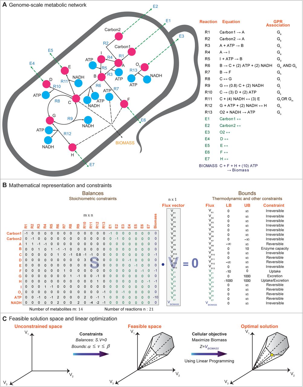
Figure 1: Vivek-Ananth, R. P., and Areejit Samal. "Advances in the integration of transcriptional regulatory information into genome-scale metabolic models." Biosystems 147 (2016): 1-10.
FBA with CORNETO#
In order to define a FBA problem, you need to know the following:
Genome-scale metabolic network: This is the prior knowledge, usually known as genome-scale metabolic models (GEMs). These models represent the metabolic network through a stoichiometric matrix, where each row represents a metabolite and each column represents a reaction. The entries in the matrix are the stoichiometric coefficients of the metabolites in the reactions. These models also contain annotations such as Gene-Protein-Rules (GPRs) and default reaction bounds.
Constraints: For each reaction, there are limits or “constraints” on the flux based on factors like enzyme capacities. Basically, it’s setting the maximum and minimum fluxes for the reactions.
Objective function: You then define an objective to optimize, like maximizing the production of a specific metabolite or maximizing growth rate.
LP Solver: Using linear programming techniques, you can find the flux distribution that meets the constraints and optimizes the objective function.
CORNETO naturally supports FBA-based problems by transforming a genome scale metabolic network into a prior knowledge graph, and then modelling the FBA problem as a network flow problem. This is the main building block for creating more complex problems, such as multicondition Sparse FBA or multicondition iMAT for context-specific reconstruction.
Using COBRApy#
Here we show how can we use COBRApy to import the textbook metabolic network and how can we import it in CORNETO. We will also compare the FBA solution from COBRApy and CORNETO.
from cobra.io import load_model

model = load_model("textbook")
len(model.metabolites), len(model.reactions)
(72, 95)
biomass_rxn = model.reactions.get_by_id("Biomass_Ecoli_core")
biomass_rxn
| Reaction identifier | Biomass_Ecoli_core |
| Name | Biomass Objective Function with GAM |
| Memory address | 0x7f132eaecf10 |
| Stoichiometry |
1.496 3pg_c + 3.7478 accoa_c + 59.81 atp_c + 0.361 e4p_c + 0.0709 f6p_c + 0.129 g3p_c + 0.205 g6p_c + 0.2557 gln__L_c + 4.9414 glu__L_c + 59.81 h2o_c + 3.547 nad_c + 13.0279 nadph_c + 1.7867 oaa_c... 1.496 3-Phospho-D-glycerate + 3.7478 Acetyl-CoA + 59.81 ATP + 0.361 D-Erythrose 4-phosphate + 0.0709 D-Fructose 6-phosphate + 0.129 Glyceraldehyde 3-phosphate + 0.205 D-Glucose 6-phosphate + 0.2557... |
| GPR | |
| Lower bound | 0.0 |
| Upper bound | 1000.0 |
solution = model.optimize()
print(solution)
<Solution 0.874 at 0x7f132e94b710>
Using CORNETO#
import numpy as np

import corneto as cn

cn.info()

|
|
from corneto.io import cobra_model_to_graph

G = cobra_model_to_graph(model)
G.shape
(72, 95)
rid = list(G.get_edges_by_attr("id", biomass_rxn.id))[0]
G.get_attr_edge(rid)
{'__edge_type': 'directed',
 'id': 'Biomass_Ecoli_core',
 '__source_attr': {'3pg_c': {'__value': np.float64(-1.496)},
  'accoa_c': {'__value': np.float64(-3.7478)},
  'atp_c': {'__value': np.float64(-59.81)},
  'e4p_c': {'__value': np.float64(-0.361)},
  'f6p_c': {'__value': np.float64(-0.0709)},
  'g3p_c': {'__value': np.float64(-0.129)},
  'g6p_c': {'__value': np.float64(-0.205)},
  'gln__L_c': {'__value': np.float64(-0.2557)},
  'glu__L_c': {'__value': np.float64(-4.9414)},
  'h2o_c': {'__value': np.float64(-59.81)},
  'nad_c': {'__value': np.float64(-3.547)},
  'nadph_c': {'__value': np.float64(-13.0279)},
  'oaa_c': {'__value': np.float64(-1.7867)},
  'pep_c': {'__value': np.float64(-0.5191)},
  'pyr_c': {'__value': np.float64(-2.8328)},
  'r5p_c': {'__value': np.float64(-0.8977)}},
 '__target_attr': {'adp_c': {'__value': np.float64(59.81)},
  'akg_c': {'__value': np.float64(4.1182)},
  'coa_c': {'__value': np.float64(3.7478)},
  'h_c': {'__value': np.float64(59.81)},
  'nadh_c': {'__value': np.float64(3.547)},
  'nadp_c': {'__value': np.float64(13.0279)},
  'pi_c': {'__value': np.float64(59.81)}},
 'default_lb': np.float64(0.0),
 'default_ub': np.float64(1000.0),
 'GPR': ''}
G.plot(layout="fdp")

from corneto.methods.future import MultiSampleFBA as FBA

d = cn.Data.from_cdict({"fba_example": {"Biomass_Ecoli_core": {"role": "objective"}}})

m = FBA()
P = m.build(G, d)
P.expr
{'_flow': _flow: Variable((95,), _flow),
 'edge_has_flux': edge_has_flux: Variable((95,), edge_has_flux, boolean=True),
 'flow': _flow: Variable((95,), _flow)}
P.solve(solver="scipy");
opt_flux = P.expr.flow[rid].value
opt_flux
np.float64(0.873921506968431)
sum(np.abs(P.expr.flow.value) >= 1e-6)
np.int64(48)
import pandas as pd

pd.DataFrame(P.expr.flow.value, index=G.get_attr_from_edges("id"), columns=["fluxes"])
| fluxes | |
|---|---|
| ACALD | -0.000000 |
| ACALDt | 0.000000 |
| ACKr | 0.000000 |
| ACONTa | 6.007250 |
| ACONTb | 6.007250 |
| ... | ... |
| TALA | 1.496984 |
| THD2 | 0.000000 |
| TKT1 | 1.496984 |
| TKT2 | 1.181498 |
| TPI | 7.477382 |
95 rows × 1 columns
G.plot(custom_edge_attr=cn.pl.flow_style(P), layout="fdp")

Sparse FBA#
m = FBA(lambda_reg=0.1)
P = m.build(G, d)
# We add a constraint to force at least 90% of optimal flux
P += P.expr.flow[rid] >= opt_flux * 0.90
P.solve(solver="highs", verbosity=1);
===============================================================================
                                     CVXPY
                                     v1.6.6
===============================================================================
-------------------------------------------------------------------------------
                                  Compilation
-------------------------------------------------------------------------------
-------------------------------------------------------------------------------
                                Numerical solver
-------------------------------------------------------------------------------
Running HiGHS 1.11.0 (git hash: 364c83a): Copyright (c) 2025 HiGHS under MIT licence terms
MIP  has 453 rows; 190 cols; 883 nonzeros; 95 integer variables (95 binary)
Coefficient ranges:
  Matrix [7e-02, 1e+03]
  Cost   [1e-01, 1e+00]
  Bound  [1e+00, 1e+00]
  RHS    [8e-01, 1e+03]
Presolving model
153 rows, 144 cols, 493 nonzeros  0s
123 rows, 123 cols, 415 nonzeros  0s
120 rows, 119 cols, 408 nonzeros  0s

Solving MIP model with:
   120 rows
   119 cols (78 binary, 0 integer, 0 implied int., 41 continuous, 0 domain fixed)
   408 nonzeros

Src: B => Branching; C => Central rounding; F => Feasibility pump; J => Feasibility jump;
     H => Heuristic; L => Sub-MIP; P => Empty MIP; R => Randomized rounding; Z => ZI Round;
     I => Shifting; S => Solve LP; T => Evaluate node; U => Unbounded; X => User solution;
     z => Trivial zero; l => Trivial lower; u => Trivial upper; p => Trivial point

        Nodes      |    B&B Tree     |            Objective Bounds              |  Dynamic Constraints |       Work
Src  Proc. InQueue |  Leaves   Expl. | BestBound       BestSol              Gap |   Cuts   InLp Confl. | LpIters     Time

         0       0         0   0.00%   -64.93809816    inf                  inf        0      0      0         0     0.0s
 S       0       0         0   0.00%   -64.93809816    3.685702492     1861.89%        0      0      0         0     0.0s
         0       0         0   0.00%   0.5684850774    3.685702492       84.58%        0      0      0        55     0.0s

2.6% inactive integer columns, restarting
Model after restart has 114 rows, 116 cols (75 bin., 0 int., 0 impl., 41 cont., 0 dom.fix.), and 394 nonzeros

         0       0         0   0.00%   1.884369605     3.685702492       48.87%       40      0      0      1201     0.2s
         0       0         0   0.00%   1.889893063     3.685702492       48.72%       40     40      0      1267     0.2s
 L       0       0         0   0.00%   2.269013228     3.685702492       38.44%     1930    133      0      1655     0.3s

2.7% inactive integer columns, restarting
Model after restart has 105 rows, 110 cols (71 bin., 0 int., 0 impl., 39 cont., 0 dom.fix.), and 364 nonzeros

         0       0         0   0.00%   2.269013228     3.685702492       38.44%       56      0      0      3012     0.6s
         0       0         0   0.00%   2.426464019     3.685702492       34.17%       56     43      0      3097     0.6s

Symmetry detection completed in 0.0s
Found 17 full orbitope(s) acting on 40 columns
 S       0       0         0   0.00%   2.628880095     3.685702492       28.67%     1573     62     12      5467     1.2s
        75       0        37 100.00%   3.685702492     3.685702492        0.00%     1576     62    576      8549     1.3s

Solving report
  Status            Optimal
  Primal bound      3.68570249247
  Dual bound        3.68570249247
  Gap               0% (tolerance: 0.01%)
  P-D integral      0.449746711088
  Solution status   feasible
                    3.68570249247 (objective)
                    0 (bound viol.)
                    2.66409116989e-12 (int. viol.)
                    0 (row viol.)
  Timing            1.31 (total)
                    0.00 (presolve)
                    0.00 (solve)
                    0.00 (postsolve)
  Max sub-MIP depth 4
  Nodes             75
  Repair LPs        0 (0 feasible; 0 iterations)
  LP iterations     8549 (total)
                    2019 (strong br.)
                    1242 (separation)
                    4180 (heuristics)
-------------------------------------------------------------------------------
                                    Summary
-------------------------------------------------------------------------------
G.plot(custom_edge_attr=cn.pl.flow_style(P), layout="fdp")

sum(P.expr.edge_has_flux.value > 0.5)
np.int64(45)
P.objectives
[objective_fba_example__12: Expression(AFFINE, UNKNOWN, ()),
 regularization_edge_has_flux: Expression(AFFINE, NONNEGATIVE, ())]
P.objectives[1].value
np.float64(45.00000000000076)