Acyclic boolean models of cell signaling (experimental)#
This guide shows the basics of modeling intracellular signaling using acyclic boolean models for multi-perturbation experiments. For this, we will use an extension of the CellNopt ILP method implemented with CORNETO.
Author: Attila Gabor (Heidelberg University, SaezLab)
Reviewers: Pablo Rodriguez Mier (Heidelberg University, SaezLab)
NOTE: This notebook is still experimental.
import corneto as cn
import corneto.methods.signal.cellnopt_ilp as cno

cn.info()

|
|
Introduction to a Boolean model#
As a first step we define start with a small network and corresponding datasets just to illustrate the concepts. The prior knowledge network of ‘G1’ contains three nodes, EGF, TNFa and Ras. Edges show the potential activation of the RAS protein.
# Definition of the prior knowledge network
G1 = cn.Graph.from_sif_tuples(
    [
        ("EGF", 1, "AND1"),
        ("TNFa", 1, "AND1"),
        ("AND1", 1, "Ras"),
        ("EGF", 1, "Ras"),
        ("TNFa", 1, "Ras"),
    ]
)
G1.plot()

Now, we organize some in-silico experimental data into a format that can be used by the CNO toolbox.
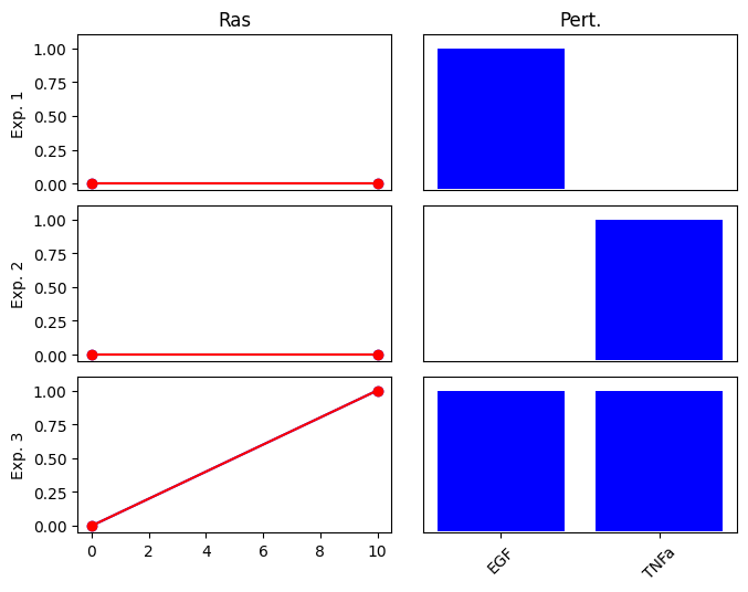
First, we define 4 conditions (exp0 … exp3). In each condition, the activated nodes (EGF or TNFa) are set to 1 and the non-activated nodes to 0. We also define the values of the corresponding outputs (Ras).
Note that the output, Ras is only active (1.0) in the 4th condition, when both of the inputs are also activated. This corresponds to an AND relationship: RAS is active only if both EGF and TNFa are activated. We expect that the optimization finds the correct subgraph of the above network, which contains only the 3 nodes with the AND gates, while individual edges from EGF and TNFa to RAS are removed.
# RAS is only active iff both EGF and TNFa are active -> we need to identify the AND gate
exp_list_G1_and = {
    "exp0": {"input": {"EGF": 0, "TNFa": 0}, "output": {"Ras": 0}},
    "exp1": {"input": {"EGF": 1, "TNFa": 0}, "output": {"Ras": 0}},
    "exp2": {"input": {"EGF": 0, "TNFa": 1}, "output": {"Ras": 0}},
    "exp3": {"input": {"EGF": 1, "TNFa": 1}, "output": {"Ras": 1}},
}
G1_prep = cno.expand_graph_for_flows(G1, exp_list_G1_and)
G1_prep.plot()

cno.plot_data(exp_list_G1_and)

P = cno.cellnoptILP(G1_prep, exp_list_G1_and, verbose=False)
cno.plot_fitness(G1, exp_list_G1_and, P, measured_only=True)
G1_prep.plot(custom_edge_attr=cno.cno_style(P, flow_name="edge_activates", scale=None, iexp=3))

Tasks:
modify the experiments so that it corresponds to a scenario where only EGF could activate RAS, but not TNFa.
modify the experiments so that it corresponds to a scenario where both TNFa or EGF could activate RAS.
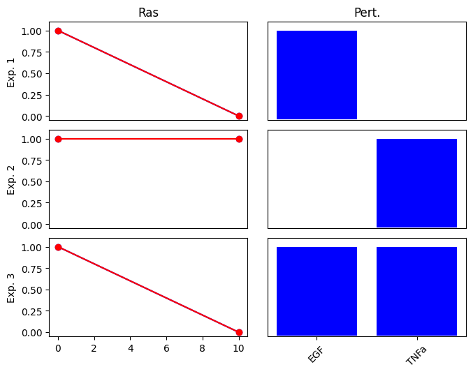
Inhibition: !EGF activates RAS#
Let’s define the same network but now we will add an inhibition of EGF on RAS. This means that if EGF is active, RAS should be inactive. Note the difference in the definition of the prior knowledge network.
We also change the experiments so that the output RAS is active only when TNFa is active.
# Test graph
G2 = cn.Graph.from_sif_tuples(
    [
        ("EGF", -1, "AND1"),
        ("TNFa", 1, "AND1"),
        ("AND1", 1, "Ras"),
        ("EGF", -1, "Ras"),
        ("TNFa", 1, "Ras"),
    ]
)

# RAS is only active iff both EGF and TNFa are active -> we need to idetify the AND gate
exp_list_G2_egf = {
    "exp0": {"input": {"EGF": 0, "TNFa": 0}, "output": {"Ras": 1}},
    "exp1": {"input": {"EGF": 1, "TNFa": 0}, "output": {"Ras": 0}},
    "exp2": {"input": {"EGF": 0, "TNFa": 1}, "output": {"Ras": 1}},
    "exp3": {"input": {"EGF": 1, "TNFa": 1}, "output": {"Ras": 0}},
}
G2_prep = cno.expand_graph_for_flows(G2, exp_list_G2_egf)
G2_prep.plot()

P2 = cno.cellnoptILP(G2_prep, exp_list_G2_egf, verbose=False)
cno.plot_fitness(G2_prep, exp_list_G2_egf, P2, measured_only=True)
G2_prep.plot(custom_edge_attr=cno.cno_style(P2, flow_name="edge_activates", scale=None, iexp=0))

Inhibition with AND gates#
Please remember, inhibitions are added to the incoming edge of the AND node. The outgoing edges of the AND node are always activating by convention.
# Test graph
G2 = cn.Graph.from_sif_tuples(
    [
        ("EGF", -1, "AND1"),
        ("TNFa", 1, "AND1"),
        ("AND1", 1, "Ras"),
        ("EGF", -1, "Ras"),
        ("TNFa", 1, "Ras"),
    ]
)

# RAS is only active iff both EGF and TNFa are active -> we need to idetify the AND gate
exp_list_G2_and = {
    "exp0": {"input": {"EGF": 0, "TNFa": 0}, "output": {"Ras": 0}},
    "exp1": {"input": {"EGF": 1, "TNFa": 0}, "output": {"Ras": 0}},
    "exp2": {"input": {"EGF": 0, "TNFa": 1}, "output": {"Ras": 1}},
    "exp3": {"input": {"EGF": 1, "TNFa": 1}, "output": {"Ras": 0}},
}
G2_prep = cno.expand_graph_for_flows(G2, exp_list_G2_and)
G2_prep.plot()
P2 = cno.cellnoptILP(G2_prep, exp_list_G2_and, verbose=False)
G2_prep.plot(custom_edge_attr=cno.cno_style(P2, flow_name="edge_activates", scale=None, iexp=2))

cno.plot_fitness(G2_prep, exp_list_G2_and, P2, measured_only=True)

Complex case study with inhibition#
Let’s look at a more realistic case study which contains a larger network and more experiments.
Also note that the we define inhibition in the experimental description. This could be, for example, the effect of small molecule kinase inhibitor.
G3 = cn.Graph.from_sif_tuples(
    [
        ("EGF", 1, "Ras"),
        ("EGF", 1, "PI3K"),
        ("TNFa", 1, "PI3K"),
        ("TNFa", 1, "TRAF6"),
        ("TRAF6", 1, "p38"),
        ("TRAF6", 1, "Jnk"),
        ("TRAF6", 1, "NFkB"),
        ("Jnk", 1, "cJun"),
        ("p38", 1, "Hsp27"),
        ("PI3K", 1, "Akt"),
        ("Ras", 1, "Raf"),
        ("Raf", 1, "Mek"),
        ("Akt", -1, "Mek"),
        ("Mek", 1, "p90RSK"),
        ("Mek", 1, "Erk"),
        ("Erk", 1, "Hsp27"),
    ]
)
# G3.add_edge((), 'EGF')
# G3.add_edge((), 'TNFa')
# G3.add_edge('Akt', ())
# G3.add_edge('cJun', ())
# G3.add_edge('Hsp27', ())
# G3.add_edge('NFkB', ())
# G3.add_edge('Erk', ())
# G3.add_edge('p90RSK', ())
# G3.add_edge('Jnk', ())

exp_list_toy_full = {
    "exp0": {
        "input": {"EGF": 0, "TNFa": 0},
        "inhibition": {},
        "output": {
            "Akt": 0,
            "Hsp27": 0,
            "NFkB": 0,
            "Erk": 0,
            "p90RSK": 0,
            "Jnk": 0,
            "cJun": 0,
        },
    },
    "exp1": {
        "input": {"EGF": 1, "TNFa": 0},
        "inhibition": {},
        "output": {
            "Akt": 0.91,
            "Hsp27": 0,
            "NFkB": 0.86,
            "Erk": 0.8,
            "p90RSK": 0.88,
            "Jnk": 0,
            "cJun": 0,
        },
    },
    "exp2": {
        "input": {"EGF": 0, "TNFa": 1},
        "inhibition": {},
        "output": {
            "Akt": 0.82,
            "Hsp27": 0.7,
            "NFkB": 0.90,
            "Erk": 0.0,
            "p90RSK": 0.0,
            "Jnk": 0.25,
            "cJun": 0.4,
        },
    },
    "exp3": {
        "input": {"EGF": 1, "TNFa": 1},
        "inhibition": {},
        "output": {
            "Akt": 0.91,
            "Hsp27": 0.7,
            "NFkB": 0.90,
            "Erk": 0.8,
            "p90RSK": 0.88,
            "Jnk": 0.25,
            "cJun": 0.4,
        },
    },
    "exp4": {
        "input": {"EGF": 1, "TNFa": 0},
        "inhibition": {"Raf": 1},
        "output": {
            "Akt": 0.91,
            "Hsp27": 0,
            "NFkB": 0.86,
            "Erk": 0.0,
            "p90RSK": 0.0,
            "Jnk": 0,
            "cJun": 0,
        },
    },
    "exp5": {
        "input": {"EGF": 0, "TNFa": 1},
        "inhibition": {"Raf": 1},
        "output": {
            "Akt": 0.82,
            "Hsp27": 0.7,
            "NFkB": 0.90,
            "Erk": 0.0,
            "p90RSK": 0.0,
            "Jnk": 0.25,
            "cJun": 0.4,
        },
    },
    "exp6": {
        "input": {"EGF": 1, "TNFa": 1},
        "inhibition": {"Raf": 1},
        "output": {
            "Akt": 0.91,
            "Hsp27": 0.7,
            "NFkB": 0.90,
            "Erk": 0.0,
            "p90RSK": 0.0,
            "Jnk": 0.25,
            "cJun": 0.4,
        },
    },
    "exp7": {
        "input": {"EGF": 1, "TNFa": 0},
        "inhibition": {"PI3K": 1},
        "output": {
            "Akt": 0.0,
            "Hsp27": 0,
            "NFkB": 0.0,
            "Erk": 0.8,
            "p90RSK": 0.88,
            "Jnk": 0,
            "cJun": 0,
        },
    },
    "exp8": {
        "input": {"EGF": 0, "TNFa": 1},
        "inhibition": {"PI3K": 1},
        "output": {
            "Akt": 0.0,
            "Hsp27": 0.7,
            "NFkB": 0.90,
            "Erk": 0.0,
            "p90RSK": 0.0,
            "Jnk": 0.25,
            "cJun": 0.4,
        },
    },
    "exp9": {
        "input": {"EGF": 1, "TNFa": 1},
        "inhibition": {"PI3K": 1},
        "output": {
            "Akt": 0.0,
            "Hsp27": 0.7,
            "NFkB": 0.90,
            "Erk": 0.8,
            "p90RSK": 0.88,
            "Jnk": 0.25,
            "cJun": 0.4,
        },
    },
}


G3.plot()

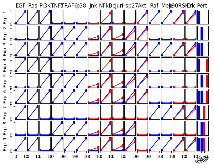
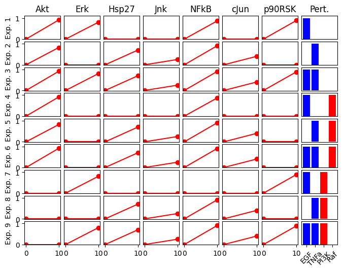
cno.plot_data(exp_list_toy_full)
G3_prep = cno.expand_graph_for_flows(G3, exp_list_toy_full)
G3_prep.plot()

P_G3 = cno.cellnoptILP(G3_prep, exp_list_toy_full, verbose=False)
---------------------------------------------------------------------------
IndexError                                Traceback (most recent call last)
Cell In[21], line 1
----> 1 P_G3 = cno.cellnoptILP(G3_prep, exp_list_toy_full, verbose=False)

File ~/work/corneto/corneto/corneto/methods/signal/cellnopt_ilp.py:265, in cellnoptILP(G, exp_list, solver, alpha_flow, verbose, backend)
    261     P += (
    262         V[is_regular_node, iexp] <= (At @ Eact)[is_regular_node, iexp]
    263     )  # but it has an upper constraint, so it takes 0 when all input are 0
    264     if V_is_inhibited[:, iexp].any():
--> 265         P += V[inh_idx[:, iexp], iexp] == np.zeros(sum(V_is_inhibited[:, iexp]))
    267 # AND relation expressed as follows:
    268 # - we only define these constraints for the AND gates
    269 # - we count the sum of flows (selected edges) and sum of activated edges
    270 # - if sum of flow equal to the sum of incoming edge activation, i.e. all edge are activated, then the vertex is activated:
    271 # - to ensure that the AND gate is not active when there is no flow (an no active edge), we add the second constraint:
    272 if V_is_and.any():
    273     # and_idx = np.flatnonzero(V_is_and)

IndexError: too many indices for array: array is 1-dimensional, but 2 were indexed
G3_prep.plot(custom_edge_attr=cno.cno_style(P_G3, flow_name="edge_activates", scale=None, iexp=3))

cno.plot_fitness(G3_prep, exp_list_toy_full, P_G3)