Multi-condition signalling network inference#
In this notebook we show how to infer signalling networks for a multicondition setting.
Here we will use mouse RNA-seq data of a multicondition study, where we will compare normal to spontaneous leukemia and Sleeping-Beauty (SB) mediated leukemia.
In the first part, we will show how to estimate Transcription Factor activities from gene expression data, following the Decoupler tutorial for functional analysis.
Then, we will infer 2 networks for each of the 2 conditions and analyse differences.
Author: Irene Rigato (Francesca Finotello’s group)
Reviewers: Sophia Müller-Dott, Pablo Rodriguez-Mier
# --- Saezlab tools ---
# https://decoupler-py.readthedocs.io/
import gzip
import os
import shutil
import tempfile
import urllib.request

import decoupler as dc
import numpy as np

# https://omnipathdb.org/
import omnipath as op

# Additional packages
import pandas as pd

# --- Additional libs ---
# Pydeseq for differential expression analysis
from pydeseq2.dds import DefaultInference, DeseqDataSet
from pydeseq2.ds import DeseqStats

# https://saezlab.github.io/
import corneto as cn

cn.info()
---------------------------------------------------------------------------
ModuleNotFoundError                       Traceback (most recent call last)
Cell In[1], line 20
     16 import pandas as pd
     18 # --- Additional libs ---
     19 # Pydeseq for differential expression analysis
---> 20 from pydeseq2.dds import DefaultInference, DeseqDataSet
     21 from pydeseq2.ds import DeseqStats
     23 # https://saezlab.github.io/

ModuleNotFoundError: No module named 'pydeseq2'
max_time = 300
seed = 0
# loading GEO GSE148679 dataset
url = "https://www.ncbi.nlm.nih.gov/geo/download/?acc=GSE148679&format=file&file=GSE148679%5Fcounts%5Fgsea%5Fanalysis%2Etxt%2Egz"

adata = None
with tempfile.TemporaryDirectory() as tmpdirname:
    # Path for the gzipped file in the temp folder
    gz_file_path = os.path.join(tmpdirname, "counts.txt.gz")

    # Download the file
    with urllib.request.urlopen(url) as response:
        with open(gz_file_path, "wb") as out_file:
            shutil.copyfileobj(response, out_file)

    # Decompress the file
    decompressed_file_path = gz_file_path[:-3]  # Removing '.gz' extension
    with gzip.open(gz_file_path, "rb") as f_in:
        with open(decompressed_file_path, "wb") as f_out:
            shutil.copyfileobj(f_in, f_out)

    adata = pd.read_csv(decompressed_file_path, index_col=0, sep="\t").T

adata.head()
| ID | Itm2a | Sergef | Fam109a | Dhx9 | Fam71e2 | Ssu72 | Olfr1018 | Eif2b2 | Mks1 | Hebp2 | ... | Olfr372 | Gosr1 | Ctsw | Ryk | Rhd | Pxmp4 | Gm25500 | 4930455C13Rik | Prss39 | Reg4 |
|---|---|---|---|---|---|---|---|---|---|---|---|---|---|---|---|---|---|---|---|---|---|
| Ebf1.1 | 265 | 332 | 306 | 27823 | 0 | 2969 | 0 | 2614 | 231 | 6 | ... | 0 | 2967 | 674 | 150 | 708 | 830 | 29 | 9 | 7 | 0 |
| Ebf1.2 | 175 | 471 | 335 | 35978 | 0 | 3108 | 0 | 2924 | 192 | 0 | ... | 0 | 2724 | 155 | 142 | 869 | 867 | 5 | 4 | 16 | 0 |
| Ebf1.3 | 266 | 382 | 325 | 30367 | 0 | 3207 | 0 | 2940 | 211 | 7 | ... | 0 | 2547 | 87 | 54 | 291 | 767 | 7 | 7 | 6 | 0 |
| Ebf1.4 | 212 | 388 | 331 | 30406 | 0 | 3168 | 0 | 2871 | 209 | 8 | ... | 0 | 2568 | 169 | 115 | 1244 | 829 | 5 | 1 | 4 | 0 |
| PE.1 | 321 | 312 | 290 | 22272 | 0 | 2631 | 0 | 2236 | 109 | 10 | ... | 0 | 2466 | 837 | 191 | 921 | 888 | 2 | 2 | 8 | 0 |
5 rows × 24420 columns
from anndata import AnnData

adata = AnnData(adata, dtype=np.float32)
adata.var_names_make_unique()
adata
AnnData object with n_obs × n_vars = 53 × 24420
# renaming conditions for clarity
adata.obs["condition"] = np.select(
    [
        adata.obs.index.str.contains("WT"),
        adata.obs.index.str.contains("Pax5"),
        adata.obs.index.str.contains("Ebf1"),
        adata.obs.index.str.contains("Leuk"),
        adata.obs.index.str.contains("SB"),
    ],
    ["Normal", "Normal", "Normal", "Leukemic_spontaneous", "Leukemic_SB"],
    default="Normal",
)
# Visualize metadata
adata.obs["condition"].value_counts()
condition
Leukemic_SB             31
Normal                  15
Leukemic_spontaneous     7
Name: count, dtype: int64
Splitting data for network inference and validation#
We will validate the network for the comparison Leukemic_SB vs Normal (enough samples)
adata1 = adata[adata.obs["condition"].isin(["Normal", "Leukemic_spontaneous"])].copy()
adata2 = adata[adata.obs["condition"].isin(["Normal", "Leukemic_SB"])].copy()
Differential expression analysis per condition#
Contrast 1: Leukemic_spontaneous vs Normal#
# Obtain genes that pass the thresholds
dc.pp.filter_by_expr(
    adata1,
    group="condition",
    min_count=10,
    min_total_count=15,
    large_n=10,
    min_prop=0.8,
)
adata1
AnnData object with n_obs × n_vars = 22 × 13585
    obs: 'condition'
# Estimation of differential expression
inference1 = DefaultInference()
dds1 = DeseqDataSet(
    adata=adata1,
    design_factors="condition",
    refit_cooks=True,
    inference=inference1,
)
dds1.deseq2()
Using None as control genes, passed at DeseqDataSet initialization
stat_res_leu1 = DeseqStats(dds1, contrast=["condition", "Leukemic_spontaneous", "Normal"], inference=inference1)

stat_res_leu1.summary()
Log2 fold change & Wald test p-value: condition Leukemic_spontaneous vs Normal
                   baseMean  log2FoldChange     lfcSE      stat        pvalue  \
ID
1810058I24Rik   2306.834064       -0.520564  0.209899 -2.480062  1.313597e-02
Lca5             588.642616       -0.161766  0.133110 -1.215284  2.242579e-01
Ndufa10         4117.949269        0.398850  0.069244  5.760057  8.408572e-09
Appbp2          2465.170707        0.118539  0.079705  1.487218  1.369574e-01
Kifc5b           690.030303       -0.424162  0.099361 -4.268891  1.964470e-05
...                     ...             ...       ...       ...           ...
Cysltr2          286.562425       -4.825286  0.629909 -7.660289  1.855156e-14
4632428C04Rik     56.421523       -2.093111  0.276118 -7.580482  3.442732e-14
Rpl3l            139.393115       -2.158983  0.363642 -5.937118  2.900761e-09
Zmym5           2503.994249       -0.176314  0.076212 -2.313479  2.069633e-02
Calr           31398.387870        0.239688  0.101100  2.370808  1.774925e-02

                       padj
ID
1810058I24Rik  1.963385e-02
Lca5           2.674048e-01
Ndufa10        2.596737e-08
Appbp2         1.710551e-01
Kifc5b         4.193482e-05
...                     ...
Cysltr2        9.467430e-14
4632428C04Rik  1.721366e-13
Rpl3l          9.335902e-09
Zmym5          3.000957e-02
Calr           2.599996e-02

[13585 rows x 6 columns]
results_df1 = stat_res_leu1.results_df
results_df1.sort_values(by="padj", ascending=True, inplace=False).head()
| baseMean | log2FoldChange | lfcSE | stat | pvalue | padj | |
|---|---|---|---|---|---|---|
| ID | ||||||
| Egfl6 | 958.998149 | -6.296339 | 0.244241 | -25.779215 | 1.516794e-146 | 1.279074e-142 |
| Polm | 2883.081884 | -7.255498 | 0.281539 | -25.770836 | 1.883068e-146 | 1.279074e-142 |
| Kdm5b | 2202.514358 | -5.510307 | 0.220788 | -24.957441 | 1.772980e-137 | 8.028642e-134 |
| Milr1 | 1647.365126 | 1.244237 | 0.050208 | 24.781408 | 1.422471e-135 | 4.831069e-132 |
| Adgre5 | 10346.763067 | -3.102891 | 0.125360 | -24.751915 | 2.956557e-135 | 8.032965e-132 |
Contrast 2: Leukemic_SB vs Normal#
# Obtain genes that pass the thresholds
dc.pp.filter_by_expr(
    adata2,
    group="condition",
    min_count=10,
    min_total_count=15,
    large_n=10,
    min_prop=0.8,
)
adata2
AnnData object with n_obs × n_vars = 46 × 13404
    obs: 'condition'
# Estimation of differential expression
inference2 = DefaultInference()
dds2 = DeseqDataSet(
    adata=adata2,
    design_factors="condition",
    refit_cooks=True,
    inference=inference2,
)
dds2.deseq2()
Using None as control genes, passed at DeseqDataSet initialization
stat_res_leu2 = DeseqStats(dds2, contrast=["condition", "Leukemic_SB", "Normal"], inference=inference2)

stat_res_leu2.summary()
Log2 fold change & Wald test p-value: condition Leukemic_SB vs Normal
                   baseMean  log2FoldChange     lfcSE       stat  \
ID
1810058I24Rik   2064.811388       -0.442806  0.118660  -3.731708
Lca5             510.125522       -0.359272  0.149948  -2.395976
Ndufa10         4456.508043        0.394199  0.090897   4.336742
Appbp2          2462.624276        0.090457  0.064445   1.403626
Kifc5b           592.263227       -0.501251  0.082228  -6.095893
...                     ...             ...       ...        ...
Cysltr2          138.715435       -5.529876  0.471282 -11.733688
4632428C04Rik     30.799835       -2.844812  0.312001  -9.117946
Rpl3l            105.987870       -1.395339  0.433373  -3.219718
Zmym5           2220.329783       -0.312692  0.074025  -4.224160
Calr           35244.098802        0.385481  0.089990   4.283597

                     pvalue          padj
ID
1810058I24Rik  1.901861e-04  4.137057e-04
Lca5           1.657617e-02  2.635358e-02
Ndufa10        1.446102e-05  3.691401e-05
Appbp2         1.604301e-01  2.067697e-01
Kifc5b         1.088284e-09  4.606051e-09
...                     ...           ...
Cysltr2        8.564356e-32  2.381673e-30
4632428C04Rik  7.656182e-20  8.495320e-19
Rpl3l          1.283169e-03  2.467662e-03
Zmym5          2.398333e-05  5.918124e-05
Calr           1.838955e-05  4.627248e-05

[13404 rows x 6 columns]
results_df2 = stat_res_leu2.results_df
results_df2.sort_values(by="padj", ascending=True, inplace=False).head()
| baseMean | log2FoldChange | lfcSE | stat | pvalue | padj | |
|---|---|---|---|---|---|---|
| ID | ||||||
| Mfsd2b | 2252.744179 | -9.412063 | 0.308793 | -30.480193 | 4.769906e-204 | 6.393582e-200 |
| Itga2b | 8434.243135 | -11.914356 | 0.401437 | -29.679285 | 1.421308e-193 | 9.525603e-190 |
| Adgrl4 | 148.349960 | -9.117488 | 0.322229 | -28.295029 | 3.978579e-176 | 1.777629e-172 |
| Gp1ba | 2396.209744 | -8.226071 | 0.323265 | -25.446856 | 7.648486e-143 | 2.563008e-139 |
| Ppbp | 17321.675345 | -15.613716 | 0.621843 | -25.108767 | 3.989417e-139 | 1.069483e-135 |
Prior knowledge with Decoupler and Omnipath#
# Retrieve CollecTRI gene regulatory network (through Omnipath)
collectri = dc.op.collectri(organism="mouse")
collectri.head()
| source | target | weight | resources | references | sign_decision | |
|---|---|---|---|---|---|---|
| 0 | Myc | Tert | 1.0 | DoRothEA-A;ExTRI;HTRI;NTNU.Curated;Pavlidis202... | 10022128;10491298;10606235;10637317;10723141;1... | PMID |
| 1 | Spi1 | Bglap3 | 1.0 | ExTRI | 10022617 | default activation |
| 2 | Spi1 | Bglap | 1.0 | ExTRI | 10022617 | default activation |
| 3 | Spi1 | Bglap2 | 1.0 | ExTRI | 10022617 | default activation |
| 4 | Smad3 | Jun | 1.0 | ExTRI;NTNU.Curated;TFactS;TRRUST | 10022869;12374795 | PMID |
TF activity inference per condition#
Contrast 1: Leukemic_spontaneous vs Normal#
mat1 = results_df1[["stat"]].T.rename(index={"stat": "Leukemic_spontaneous.vs.Normal"})
mat1
| ID | 1810058I24Rik | Lca5 | Ndufa10 | Appbp2 | Kifc5b | Dusp14 | Snx13 | Hdhd3 | Dnajb14 | Tesk2 | ... | Emc7 | B3galt5 | Tmprss4 | Kif4 | Alpk2 | Cysltr2 | 4632428C04Rik | Rpl3l | Zmym5 | Calr |
|---|---|---|---|---|---|---|---|---|---|---|---|---|---|---|---|---|---|---|---|---|---|
| Leukemic_spontaneous.vs.Normal | -2.480062 | -1.215284 | 5.760057 | 1.487218 | -4.268891 | -4.893978 | -0.736225 | 3.792193 | -2.018379 | -9.098806 | ... | 1.907317 | 2.085353 | 9.76056 | -10.189153 | -1.853138 | -7.660289 | -7.580482 | -5.937118 | -2.313479 | 2.370808 |
1 rows × 13585 columns
tf_acts1, tf_pvals1 = dc.mt.ulm(data=mat1, net=collectri, verbose=True)
tf_acts1
| Abl1 | Ahr | Aire | Apex1 | Ar | Arid1a | Arid1b | Arid3a | Arid3b | Arid4a | ... | Zfpm1 | Zfpm2 | Zglp1 | Zgpat | Zhx2 | Zic1 | Zic2 | Zkscan3 | Zkscan4 | Zkscan7 | |
|---|---|---|---|---|---|---|---|---|---|---|---|---|---|---|---|---|---|---|---|---|---|
| Leukemic_spontaneous.vs.Normal | 1.452444 | -0.115657 | -2.245577 | 0.882836 | -0.298509 | -0.176434 | -0.632351 | -0.453507 | -1.821614 | 0.260513 | ... | -1.43915 | 0.110719 | -1.527694 | -0.947716 | 1.092937 | 0.530854 | -0.030247 | 1.945875 | 1.945875 | 1.025677 |
1 rows × 640 columns
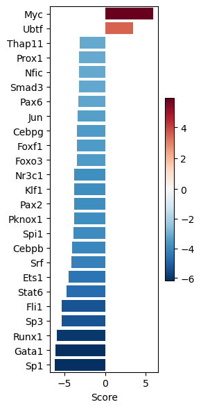
dc.pl.barplot(
    data=tf_acts1,
    name="Leukemic_spontaneous.vs.Normal",
    top=25,
    figsize=(3, 6),
)
Contrast 2: Leukemic_SB vs Normal#
mat2 = results_df2[["stat"]].T.rename(index={"stat": "Leukemic_SB.vs.Normal"})
mat2
| ID | 1810058I24Rik | Lca5 | Ndufa10 | Appbp2 | Kifc5b | Snx13 | Hdhd3 | Dnajb14 | Tesk2 | Adnp | ... | Emc7 | B3galt5 | Tmprss4 | Kif4 | Alpk2 | Cysltr2 | 4632428C04Rik | Rpl3l | Zmym5 | Calr |
|---|---|---|---|---|---|---|---|---|---|---|---|---|---|---|---|---|---|---|---|---|---|
| Leukemic_SB.vs.Normal | -3.731708 | -2.395976 | 4.336742 | 1.403626 | -6.095893 | -0.045633 | 6.58726 | 1.804979 | -4.887532 | 1.097428 | ... | 2.795666 | 3.052277 | 6.874866 | -9.738949 | 1.052295 | -11.733688 | -9.117946 | -3.219718 | -4.22416 | 4.283597 |
1 rows × 13404 columns
tf_acts2, tf_pvals2 = dc.mt.ulm(data=mat2, net=collectri, verbose=True)
tf_acts2
| Abl1 | Ahr | Aire | Apex1 | Ar | Arid1a | Arid1b | Arid3a | Arid3b | Arid4a | ... | Zfpm1 | Zfpm2 | Zglp1 | Zgpat | Zhx2 | Zic1 | Zic2 | Zkscan3 | Zkscan4 | Zkscan7 | |
|---|---|---|---|---|---|---|---|---|---|---|---|---|---|---|---|---|---|---|---|---|---|
| Leukemic_SB.vs.Normal | 1.198683 | 0.664987 | -0.932035 | 1.417199 | 0.441126 | 0.676737 | -1.148896 | -0.229277 | -1.489196 | 0.92969 | ... | -1.618176 | -0.165154 | -0.623824 | -1.382751 | 1.35549 | 0.659029 | -0.049623 | 1.390877 | 1.390877 | 1.316184 |
1 rows × 625 columns
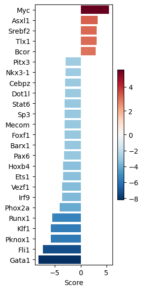
dc.pl.barplot(
    data=tf_acts2,
    name="Leukemic_SB.vs.Normal",
    top=25,
    figsize=(3, 6),
)
Retrieving potential receptors per condition#
# We obtain ligand-receptor interactions from Omnipath, and we keep only the receptors
# This is our list of a prior potential receptors from which we will infer the network
unique_receptors = set(
    op.interactions.LigRecExtra.get(organisms="mouse", genesymbols=True)["target_genesymbol"].values.tolist()
)
len(unique_receptors)
849
Contrast 1: Leukemic_spontaneous vs Normal#
df_de_receptors1 = results_df1.loc[results_df1.index.intersection(unique_receptors)]
df_de_receptors1 = df_de_receptors1.sort_values(by="stat", ascending=False)
# We will take the top 20 receptors that increased the expression after treatment
df_top_receptors1 = df_de_receptors1.head(30)
df_top_receptors1.head()
| baseMean | log2FoldChange | lfcSE | stat | pvalue | padj | |
|---|---|---|---|---|---|---|
| ID | ||||||
| Mrc1 | 314.324326 | 3.312083 | 0.179667 | 18.434602 | 6.932705e-76 | 2.943150e-73 |
| St14 | 1073.819725 | 1.904158 | 0.116095 | 16.401736 | 1.858495e-60 | 3.078982e-58 |
| Cd48 | 5533.470898 | 0.664655 | 0.054604 | 12.172306 | 4.365699e-34 | 1.215328e-32 |
| Ifngr1 | 6551.268902 | 1.418280 | 0.120961 | 11.725146 | 9.473804e-32 | 2.181384e-30 |
| Lrrc4c | 82.859784 | 10.019258 | 0.895652 | 11.186547 | 4.745541e-29 | 8.584311e-28 |
Contrast 2: Leukemic_SB vs Normal#
df_de_receptors2 = results_df2.loc[results_df2.index.intersection(unique_receptors)]
df_de_receptors2 = df_de_receptors2.sort_values(by="stat", ascending=False)
# We will take the top 20 receptors that increased the expression after treatment
df_top_receptors2 = df_de_receptors2.head(30)
df_top_receptors2.head()
| baseMean | log2FoldChange | lfcSE | stat | pvalue | padj | |
|---|---|---|---|---|---|---|
| ID | ||||||
| Lsr | 770.417182 | 4.360408 | 0.346097 | 12.598814 | 2.143445e-36 | 8.425435e-35 |
| Ptprs | 5164.424536 | 1.303309 | 0.109463 | 11.906393 | 1.096177e-32 | 3.257906e-31 |
| Nlgn2 | 1309.701665 | 1.950302 | 0.165263 | 11.801208 | 3.847470e-32 | 1.106684e-30 |
| Cd244 | 2529.473998 | 2.992844 | 0.255033 | 11.735143 | 8.418380e-32 | 2.345945e-30 |
| Lrrc4c | 267.125842 | 10.650499 | 0.916744 | 11.617743 | 3.348651e-31 | 8.783820e-30 |
Inferring intracellular signalling network with CORNETO#
cn.info()

|
|
from corneto.methods.future import CarnivalFlow

# CarnivalFlow.show_citations()
Setting prior knowledge graph#
pkn = op.interactions.OmniPath.get(organisms="mouse", databases=["SIGNOR"], genesymbols=True)
pkn = pkn[pkn.consensus_direction == True]
pkn.head()
| source | target | source_genesymbol | target_genesymbol | is_directed | is_stimulation | is_inhibition | consensus_direction | consensus_stimulation | consensus_inhibition | curation_effort | references | sources | n_sources | n_primary_sources | n_references | references_stripped | |
|---|---|---|---|---|---|---|---|---|---|---|---|---|---|---|---|---|---|
| 0 | P0C605 | Q9QZC1 | Prkg1 | Trpc3 | True | False | True | True | False | True | 9 | HPRD:14983059;KEA:14983059;ProtMapper:14983059... | HPRD;HPRD_KEA;HPRD_MIMP;KEA;MIMP;PhosphoPoint;... | 15 | 8 | 2 | 14983059;16331690 |
| 1 | P0C605 | Q9WVC5 | Prkg1 | Trpc7 | True | True | False | True | True | False | 3 | SIGNOR:21402151;TRIP:21402151;iPTMnet:21402151 | SIGNOR;TRIP;iPTMnet | 3 | 3 | 1 | 21402151 |
| 2 | Q8K2C7 | Q9EPK8 | Os9 | Trpv4 | True | True | True | True | True | True | 3 | HPRD:17932042;SIGNOR:17932042;TRIP:17932042 | HPRD;SIGNOR;TRIP | 3 | 3 | 1 | 17932042 |
| 3 | P35821 | Q91WD2 | Ptpn1 | Trpv6 | True | False | True | True | False | True | 11 | DEPOD:15894168;DEPOD:17197020;HPRD:15894168;In... | DEPOD;HPRD;IntAct;Lit-BM-17;SIGNOR;SPIKE_LC;TRIP | 7 | 6 | 2 | 15894168;17197020 |
| 4 | P68040 | Q8CIR4 | Rack1 | Trpm6 | True | False | True | True | False | True | 2 | SIGNOR:18258429;TRIP:18258429 | SIGNOR;TRIP | 2 | 2 | 1 | 18258429 |
pkn["interaction"] = pkn["is_stimulation"].astype(int) - pkn["is_inhibition"].astype(int)
sel_pkn = pkn[["source_genesymbol", "interaction", "target_genesymbol"]]
sel_pkn.head()
| source_genesymbol | interaction | target_genesymbol | |
|---|---|---|---|
| 0 | Prkg1 | -1 | Trpc3 |
| 1 | Prkg1 | 1 | Trpc7 |
| 2 | Os9 | 0 | Trpv4 |
| 3 | Ptpn1 | -1 | Trpv6 |
| 4 | Rack1 | -1 | Trpm6 |
# We create the CORNETO graph by importing the edges and interaction
G = cn.Graph.from_sif_tuples([(r[0], r[1], r[2]) for _, r in sel_pkn.iterrows() if r[1] != 0])
G.shape  # nodes, edges
(4304, 9505)
Identifying target TFs per condition#
max_pval = 0.01
Contrast 1: Leukemic_spontaneous vs Normal#
# As measurements, we take the estimated TFs, we will filter out TFs with p-val > 0.001
significant_tfs1 = (
    tf_acts1[tf_pvals1 <= max_pval].T.dropna().sort_values(by="Leukemic_spontaneous.vs.Normal", ascending=False)
)
significant_tfs1.head()
| Leukemic_spontaneous.vs.Normal | |
|---|---|
| Myc | 5.923504 |
| Nr3c1 | -3.811319 |
| Klf1 | -3.827703 |
| Pax2 | -3.833334 |
| Pknox1 | -3.854036 |
# We keep only the ones in the PKN graph
measurements1 = significant_tfs1.loc[significant_tfs1.index.intersection(G.V)].to_dict()[
    "Leukemic_spontaneous.vs.Normal"
]
measurements1
{'Myc': 5.9235035317894855,
 'Nr3c1': -3.8113193546675745,
 'Pax2': -3.833334174850489,
 'Pknox1': -3.8540363164880644,
 'Spi1': -3.8784486226011565,
 'Cebpb': -4.040106259374742,
 'Srf': -4.189355333236107,
 'Ets1': -4.531331302590852,
 'Stat6': -4.773632881709543,
 'Fli1': -5.33776968520547,
 'Sp3': -5.344046528477468,
 'Runx1': -5.974558044625292,
 'Gata1': -6.145310061493243,
 'Sp1': -6.183198826931179}
Contrast 2: Leukemic_SB vs Normal#
# As measurements, we take the estimated TFs, we will filter out TFs with p-val > 0.001
significant_tfs2 = tf_acts2[tf_pvals2 <= max_pval].T.dropna().sort_values(by="Leukemic_SB.vs.Normal", ascending=False)
significant_tfs2.head()
| Leukemic_SB.vs.Normal | |
|---|---|
| Myc | 5.455686 |
| Phox2a | -4.102661 |
| Runx1 | -5.481558 |
| Klf1 | -5.749639 |
| Pknox1 | -5.823607 |
# We keep only the ones in the PKN graph
measurements2 = significant_tfs2.loc[significant_tfs2.index.intersection(G.V)].to_dict()["Leukemic_SB.vs.Normal"]
measurements2
{'Myc': 5.4556864114528985,
 'Phox2a': -4.102661149717304,
 'Runx1': -5.481558125441376,
 'Pknox1': -5.823606769114178,
 'Fli1': -7.269739674233043,
 'Gata1': -8.17854383650117}
def balance_dicts_by_top_abs(dict1, dict2, discretize=False):
    # Decide which is smaller and which is larger
    if len(dict1) <= len(dict2):
        small, large = dict1, dict2
    else:
        small, large = dict2, dict1

    n = len(small)
    # Take the n keys from large with the largest abs(values)
    top_large_items = sorted(large.items(), key=lambda kv: abs(kv[1]), reverse=True)[:n]

    # Prepare output dicts
    small_balanced = dict(small)  # already of size n
    large_balanced = dict(top_large_items)

    if discretize:
        small_balanced = {k: np.sign(v) for k, v in small_balanced.items()}
        large_balanced = {k: np.sign(v) for k, v in large_balanced.items()}

    return small_balanced, large_balanced


# Discretize not needed, but simplifies multi-cond analysis since both conditions have the same cost
d_measurements1, d_measurements2 = balance_dicts_by_top_abs(measurements1, measurements2, discretize=True)
d_measurements1
{'Myc': np.float64(1.0),
 'Phox2a': np.float64(-1.0),
 'Runx1': np.float64(-1.0),
 'Pknox1': np.float64(-1.0),
 'Fli1': np.float64(-1.0),
 'Gata1': np.float64(-1.0)}
d_measurements2
{'Sp1': np.float64(-1.0),
 'Gata1': np.float64(-1.0),
 'Runx1': np.float64(-1.0),
 'Myc': np.float64(1.0),
 'Sp3': np.float64(-1.0),
 'Fli1': np.float64(-1.0)}
Creating a CARNIVAL problem per condition#
Contrast 1: Leukemic_spontaneous vs Normal#
# We will infer the direction, so for the inputs, we use a value of 0 (=unknown direction)
inputs1 = {k: 0 for k in df_top_receptors1.index.intersection(G.V).values}
inputs1
{'Ifngr1': 0,
 'Lrrc4c': 0,
 'Tnfrsf11a': 0,
 'Cdon': 0,
 'Notch1': 0,
 'Ptprs': 0,
 'Nlgn2': 0,
 'Flt3': 0,
 'Ephb4': 0,
 'Il2rg': 0,
 'Marco': 0,
 'Axl': 0,
 'Tlr4': 0,
 'Ifngr2': 0,
 'Znrf3': 0}
# Create the dataset in standard format
carnival_data1 = dict()
for inp, v in inputs1.items():
    carnival_data1[inp] = dict(value=v, role="input", mapping="vertex")
for out, v in d_measurements1.items():
    carnival_data1[out] = dict(value=v, role="output", mapping="vertex")
data1 = cn.Data.from_cdict({"sample1": carnival_data1})
data1
Data(n_samples=1, n_feats=[21])
Contrast 2: Leukemic_SB vs Normal#
# We will infer the direction, so for the inputs, we use a value of 0 (=unknown direction)
inputs2 = {k: 0 for k in df_top_receptors2.index.intersection(G.V).values}
inputs2
{'Ptprs': 0,
 'Nlgn2': 0,
 'Lrrc4c': 0,
 'Tnfrsf11a': 0,
 'Ifngr1': 0,
 'Marco': 0,
 'Ifngr2': 0,
 'Ctla4': 0,
 'Znrf3': 0,
 'Flt3': 0,
 'Ephb4': 0,
 'Il9r': 0,
 'Icam1': 0,
 'Axl': 0}
# Create the dataset in standard format
carnival_data2 = dict()
for inp, v in inputs2.items():
    carnival_data2[inp] = dict(value=v, role="input", mapping="vertex")
for out, v in d_measurements2.items():
    carnival_data2[out] = dict(value=v, role="output", mapping="vertex")
data2 = cn.Data.from_cdict({"sample2": carnival_data2})
data2
Data(n_samples=1, n_feats=[20])
Solving multi-condition CARNIVAL problem with CORNETO#
data = cn.Data.from_cdict({"sample1": carnival_data1, "sample2": carnival_data2})
data
Data(n_samples=2, n_feats=[21 20])
from corneto.utils import check_gurobi

check_gurobi()
Gurobipy successfully imported.
Gurobi environment started successfully.
Starting optimization of the test model...
Test optimization was successful.
Gurobi environment disposed.
Gurobi is correctly installed and working.
True
def subgraph(G, inp, out):
    inp_s = set(G.V).intersection(inp)
    out_s = set(G.V).intersection(out)
    Gs = G.prune(inp_s, out_s)
    tot_inp = set(Gs.V).intersection(inp)
    tot_out = set(Gs.V).intersection(out)
    print(f"Inputs: ({len(tot_inp)}/{len(inp)}), Outputs: ({len(tot_out)}/{len(out)})")
    return Gs


Gs1 = subgraph(G, df_top_receptors1.index.tolist(), list(d_measurements1.keys()))
Gs2 = subgraph(G, df_top_receptors2.index.tolist(), list(d_measurements2.keys()))
Inputs: (7/30), Outputs: (5/6)
Inputs: (4/30), Outputs: (6/6)
c = CarnivalFlow(lambda_reg=0, indirect_rule_penalty=1)
P = c.build(G, data)
Unreachable vertices for sample: 12
Unreachable vertices for sample: 7
len(set(c.processed_graph.V).intersection(d_measurements1.keys()))
5
len(set(c.processed_graph.V).intersection(d_measurements2.keys()))
6
# How many TFs are in common between conditions?
s1 = set(c.processed_graph.V).intersection(d_measurements1.keys())
s2 = set(c.processed_graph.V).intersection(d_measurements2.keys())
for g in s1.intersection(s2):
    print(g, d_measurements1[g], d_measurements2[g])
Gata1 -1.0 -1.0
Fli1 -1.0 -1.0
Runx1 -1.0 -1.0
Myc 1.0 1.0
Which is the best lambda to choose?#
To choose a robust value of \(\lambda\) we sample multiple solutions, as in the tutorial https://saezlab.github.io/corneto/dev/tutorials/network-sampler.html#vertex-based-perturbation.
We define 3 metrics to choose \(\lambda\):
\(sign\_agreement\_ratio = \frac{n.\:of\:nodes\:matching\:sign\:with\:stat\:value}{total\:n.\:of\:nodes}\)
\(de\_overlap\_ratio = \frac{n.\:of\:nodes\:also\:differentially\:expressed}{total\:n.\:of\:nodes}\)
\(overall\_agreement = \frac{sign\_agreement\_ratio\:+\:de\_overlap\_ratio}{2}\)
# retrieving alternative network solutions. This snippet will take a while to run
from corneto.methods.sampler import sample_alternative_solutions

lambda_val = [0, 0.01, 0.1, 0.2, 0.3, 0.5, 0.7, 0.9, 0.95]
other_optimal_v = dict()  # collecting the vertex sampled solutions for each lambda
index = dict()
for i in lambda_val:
    print("lambda: ", i)
    c = CarnivalFlow(lambda_reg=i, indirect_rule_penalty=1)
    P = c.build(G, data)
    vertex_results = sample_alternative_solutions(
        P,
        "vertex_value",
        percentage=0.03,
        scale=0.03,
        rel_opt_tol=0.05,
        max_samples=30,  # number of alternative solutions to sample
        solver_kwargs=dict(solver="gurobi", max_seconds=max_time, mip_gap=0.01, seed=seed),
    )
    other_optimal_v["lambda" + str(i)] = vertex_results["vertex_value"]
    index["lambda" + str(i)] = c.processed_graph.V
lambda:  0
Unreachable vertices for sample: 12
Unreachable vertices for sample: 7
Set parameter Username
Set parameter LicenseID to value 2593994
Academic license - for non-commercial use only - expires 2025-12-02
lambda:  0.01
Unreachable vertices for sample: 12
Unreachable vertices for sample: 7
def compute_nodes_metrics(nodes, inputs, measurements, results_df, column):
    """Computes the metrics for the nodes in the network based on the provided inputs, measurements, and results dataframe.

    Args:
        nodes (pd.DataFrame): data frame containing the node scores per condition.
        inputs (dict): Dictionary of input nodes with their values.
        measurements (dict): Dictionary of output nodes with their values.
        results_df (pd.DataFrame): DataFrame containing the results of differential expression analysis.
        column (str): Column name to be used for filtering conditions.

    Returns:
        sign_agreement_ratio (float): Ratio of nodes with the same sign as the DE analysis.
        de_overlap_ratio (float): Ratio of DE genes that overlap with the nodes.
        overall_agreement (float): Overall agreement between DE genes and nodes.
    """
    nodes = nodes.loc[(nodes[column] != 0.0)][column]  # nodes with a score different from 0
    de = results_df.loc[results_df["padj"] < 0.05].index.tolist()  # de genes
    in_out_nodes = set(measurements.keys()).union(
        set(nodes.index[nodes.index.isin(inputs.keys())])
    )  # collecting input and output nodes which we don´t want to evaluate
    middle_nodes = set(nodes.index).difference(in_out_nodes)
    commmon_genes = list(
        set(results_df.index).intersection(middle_nodes)
    )  # common genes between network and DE analysis genes
    stat = results_df.loc[commmon_genes, "stat"]
    stat_sign = np.sign(stat)
    middle_nodes_sign = np.sign(nodes.loc[commmon_genes])
    sign_agreement_ratio = 0
    if len(middle_nodes_sign) > 0:
        sign_agreement_ratio = (middle_nodes_sign == stat_sign).sum() / len(middle_nodes_sign)
    de_overlap_ratio = 0
    if len(middle_nodes) > 0:
        de_overlap_ratio = len(set(de).intersection(middle_nodes)) / len(middle_nodes)
    overall_agreement = (np.array(de_overlap_ratio) + np.array(sign_agreement_ratio)) / 2

    return sign_agreement_ratio, de_overlap_ratio, overall_agreement
# Initialize metric containers
metrics_avg_1_per_lambda = []
metrics_avg_2_per_lambda = []
metrics_sd_1_per_lambda = []
metrics_sd_2_per_lambda = []

for k in other_optimal_v.keys():
    metrics1_per_sample = []
    metrics2_per_sample = []

    for i in range(len(other_optimal_v[k])):
        n = pd.DataFrame(
            other_optimal_v[k][i],
            index=index[k],
            columns=["vertex_activity1", "vertex_activity2"],
        )  # retrieving node scores

        sign_agreement1, de_overlap1, overall_agreement1 = compute_nodes_metrics(
            n, inputs1, d_measurements1, results_df1, "vertex_activity1"
        )
        sign_agreement2, de_overlap2, overall_agreement2 = compute_nodes_metrics(
            n, inputs2, d_measurements2, results_df2, "vertex_activity2"
        )

        metrics1_per_sample.append(
            {
                "sign_agreement": sign_agreement1,
                "de_overlap": de_overlap1,
                "overall": overall_agreement1,
            }
        )
        metrics2_per_sample.append(
            {
                "sign_agreement": sign_agreement2,
                "de_overlap": de_overlap2,
                "overall": overall_agreement2,
            }
        )

    metrics1_per_sample_df = pd.DataFrame(metrics1_per_sample)
    metrics2_per_sample_df = pd.DataFrame(metrics2_per_sample)
    metrics_avg_1_per_lambda.append(metrics1_per_sample_df.mean().to_dict())
    metrics_avg_2_per_lambda.append(metrics2_per_sample_df.mean().to_dict())
    metrics_sd_1_per_lambda.append(metrics1_per_sample_df.std().to_dict())
    metrics_sd_2_per_lambda.append(metrics2_per_sample_df.std().to_dict())

# Convert lists of dictionaries to DataFrames
m_avg_df1 = pd.DataFrame(metrics_avg_1_per_lambda)
m_avg_df2 = pd.DataFrame(metrics_avg_2_per_lambda)
m_sd_df1 = pd.DataFrame(metrics_sd_1_per_lambda)
m_sd_df2 = pd.DataFrame(metrics_sd_2_per_lambda)

##plotting metrics
import matplotlib.pyplot as plt

metric_name = ["sign_agreement", "de_overlap", "overall"]
metric_label = ["Sign agreement ratio", "DE overlap ratio", "Overall agreement"]

fig, axes = plt.subplots(1, 3, figsize=(25, 5), sharex=True)
for i in range(len(metric_name)):
    axes[i].errorbar(
        lambda_val,
        m_avg_df1[metric_name[i]],
        yerr=m_sd_df1[metric_name[i]],
        label="Leukemic_spontaneous",
        marker="o",
    )
    axes[i].errorbar(
        lambda_val,
        m_avg_df2[metric_name[i]],
        yerr=m_sd_df2[metric_name[i]],
        label="Leukemic_SB",
        marker="o",
    )
    axes[i].grid()
    axes[i].set_xscale("linear")  # adjust scale according to your results
    axes[i].set_xlabel("Lambda")
    axes[i].set_ylabel(metric_label[i])
    axes[i].set_title(metric_label[i] + " vs Lambda")
    if i == 0:
        axes[i].legend(loc="upper left")
We choose the lambda value basing on the Overall agreement metric. In this case a reasonable value of \(\lambda\) is 2
c = CarnivalFlow(lambda_reg=0.5, indirect_rule_penalty=1)
P = c.build(G, data)

# Optimal solutions are found when Gap is close to 0
P.solve(solver="GUROBI", verbosity=1)
# optimization metrics
for o in P.objectives:
    print(o.name, o.value)
# having a look to edge values per condition
pd.DataFrame(
    P.expr.edge_value.value,
    index=c.processed_graph.E,
    columns=["edge_activity1", "edge_activity2"],
).head(5)
# having a look to node values per condition
pd.DataFrame(
    P.expr.vertex_value.value,
    index=c.processed_graph.V,
    columns=["vertex_activity1", "vertex_activity2"],
).head(5)
Inferred network for contrast 1: Leukemic_spontaneous vs Normal#
sol_edges1 = np.flatnonzero(np.abs(P.expr.edge_value.value[:, 0]) > 0.5)
c.processed_graph.plot_values(
    vertex_values=P.expr.vertex_value.value[:, 0],
    edge_values=P.expr.edge_value.value[:, 0],
    edge_indexes=sol_edges1,
)
Inferred network for contrast 2: Leukemic_SB vs Normal#
sol_edges2 = np.flatnonzero(np.abs(P.expr.edge_value.value[:, 1]) > 0.5)
c.processed_graph.plot_values(
    vertex_values=P.expr.vertex_value.value[:, 1],
    edge_values=P.expr.edge_value.value[:, 1],
    edge_indexes=sol_edges2,
)