Exploring alternative solutions with \(\epsilon\)-perturbation sampling#
CORNETO includes a basic ε-Perturbation Sampling method for uncovering near-optimal alternatives. Starting from the optimal solution, it applies small random “jitter” to a selected variable, re-solves the model, and retains only those samples whose original objectives remain within a user-specified tolerance. The result is a collection of feasible alternatives that highlights which components are fixed versus flexible.
We will illustrate this process using a simple example of a network inference problem with CARNIVAL, using the data from the CARNIVAL transcriptomics tutorial.
NOTE: This notebook uses
gurobias the solver andcvxpyas the backend to accelerate the generation of alternative solutions using thewarm_startoption from cvxpy
import numpy as np
import pandas as pd

import corneto as cn

cn.enable_logging()
cn.info()

|
|
# Load dataset from tutorial
dataset = cn.GraphData.load("data/carnival_transcriptomics_dataset.zip")
from corneto.methods.future import CarnivalFlow

m = CarnivalFlow(lambda_reg=0.1)
P = m.build(dataset.graph, dataset.data)
P.objectives
Unreachable vertices for sample: 0
[error_sample1_0: Expression(AFFINE, UNKNOWN, ()),
 regularization_edge_has_signal: Expression(AFFINE, NONNEGATIVE, ())]
# We will sample solutions by perturbing the edge_has_signal variable
P.expr
{'_flow': _flow: Variable((3374,), _flow),
 'edge_activates': edge_activates: Variable((3374, 1), edge_activates, boolean=True),
 'const0x144be068ae3d485b': const0x144be068ae3d485b: Constant(CONSTANT, NONNEGATIVE, (970, 3374)),
 '_dag_layer': _dag_layer: Variable((970, 1), _dag_layer),
 'edge_inhibits': edge_inhibits: Variable((3374, 1), edge_inhibits, boolean=True),
 'const0x4db7440b66998bb': const0x4db7440b66998bb: Constant(CONSTANT, NONNEGATIVE, (970, 3374)),
 'flow': _flow: Variable((3374,), _flow),
 'vertex_value': Expression(AFFINE, UNKNOWN, (970, 1)),
 'vertex_activated': Expression(AFFINE, NONNEGATIVE, (970, 1)),
 'vertex_inhibited': Expression(AFFINE, NONNEGATIVE, (970, 1)),
 'edge_value': Expression(AFFINE, UNKNOWN, (3374, 1)),
 'edge_has_signal': Expression(AFFINE, NONNEGATIVE, (3374, 1))}
# These are the original objectives of the problem
for o in P.objectives:
    print(o.name)
error_sample1_0
regularization_edge_has_signal
Edge-Based Perturbation#
First, we’ll sample solutions by perturbing the edge variables. This allows us to explore alternative network topologies where different edges might be selected.
from corneto.methods.sampler import sample_alternative_solutions

# Create a fresh model
m = CarnivalFlow(lambda_reg=0.1)
P = m.build(dataset.graph, dataset.data)

# NOTE: The sampler modifies the original P problem
results = sample_alternative_solutions(
    P,
    "edge_has_signal",
    percentage=0.10,
    scale=0.05,
    rel_opt_tol=0.10,
    max_samples=30,
    solver_kwargs=dict(solver="gurobi", max_seconds=300),
)
Unreachable vertices for sample: 0
Set parameter Username
Set parameter LicenseID to value 2593994
Academic license - for non-commercial use only - expires 2025-12-02
edges = np.squeeze(results["edge_value"]).T
df_sols = pd.DataFrame(edges, index=m.processed_graph.E).astype(int)
print(f"Generated {df_sols.shape[1]} alternative solutions")
df_sols.head()
Generated 31 alternative solutions
| 0 | 1 | 2 | 3 | 4 | 5 | 6 | 7 | 8 | 9 | ... | 21 | 22 | 23 | 24 | 25 | 26 | 27 | 28 | 29 | 30 | ||
|---|---|---|---|---|---|---|---|---|---|---|---|---|---|---|---|---|---|---|---|---|---|---|
| (SMAD3) | (MYOD1) | 0 | 0 | 0 | 0 | 0 | 0 | 0 | 0 | 0 | 0 | ... | 0 | 0 | 0 | 0 | 0 | 0 | 0 | 0 | 0 | 0 |
| (GRK2) | (BDKRB2) | 0 | 0 | 0 | 0 | 0 | 0 | 0 | 0 | 0 | 0 | ... | 0 | 0 | 0 | 0 | 0 | 0 | 0 | 0 | 0 | 0 |
| (MAPK14) | (MAPKAPK2) | 0 | 0 | 0 | 0 | 0 | 0 | 0 | 0 | 0 | 0 | ... | 0 | 0 | 0 | 0 | 0 | 0 | 0 | 0 | 0 | 0 |
| (DEPTOR_EEF1A1_MLST8_MTOR_PRR5_RICTOR) | (FBXW8) | 0 | 0 | 0 | 0 | 0 | 0 | 0 | 0 | 0 | 0 | ... | 0 | 0 | 0 | 0 | 0 | 0 | 0 | 0 | 0 | 0 |
| (SLK) | (MAP3K5) | 0 | 0 | 0 | 0 | 0 | 0 | 0 | 0 | 0 | 0 | ... | 0 | 0 | 0 | 0 | 0 | 0 | 0 | 0 | 0 | 0 |
5 rows × 31 columns
# Analyze variability in edge selection
df_var = pd.concat([df_sols.mean(axis=1), df_sols.std(axis=1)], axis=1)
df_var.columns = ["mean", "std"]
print("Edges with highest variability across solutions:")
df_var.sort_values(by="std", ascending=False).head(50).sort_values(by="mean")
Edges with highest variability across solutions:
| mean | std | ||
|---|---|---|---|
| (MAPK14) | (GSK3B) | -0.741935 | 0.444803 |
| (PPP2CA) | (PRKCD) | -0.709677 | 0.461414 |
| (JUN) | (SPI1) | -0.709677 | 0.461414 |
| (GSK3B) | (CEBPA) | -0.709677 | 0.461414 |
| (TGFB1) | (PPP2R2A) | -0.677419 | 0.475191 |
| (CSNK1D) | (WWTR1) | -0.677419 | 0.475191 |
| () | (TGFB1) | -0.677419 | 0.475191 |
| (SMAD3) | (NKX2-1) | -0.645161 | 0.486373 |
| (PHLPP1) | (PRKCA) | -0.580645 | 0.501610 |
| (NFKB1_RELA) | (EGR1) | -0.548387 | 0.505879 |
| (RARG) | (RXRB) | -0.548387 | 0.505879 |
| (MAPK8) | (IRF3) | -0.548387 | 0.505879 |
| (THRA) | (RARG) | -0.548387 | 0.505879 |
| (CDK1) | (CDC25A) | -0.548387 | 0.505879 |
| (PRKCA) | (NFE2L2) | -0.516129 | 0.508001 |
| (PRKCD) | (NFE2L2) | -0.483871 | 0.508001 |
| (MAPK8) | (STAT1) | -0.483871 | 0.508001 |
| (PRKCD) | (STAT1) | -0.483871 | 0.508001 |
| (RARB) | (RXRB) | -0.451613 | 0.505879 |
| (THRA) | (RARB) | -0.451613 | 0.505879 |
| (RELA) | (EGR1) | -0.451613 | 0.505879 |
| (TBK1) | (IRF3) | -0.387097 | 0.495138 |
| (CDK1) | (TP53) | -0.354839 | 0.486373 |
| (WWTR1) | (NKX2-1) | -0.354839 | 0.486373 |
| (MAPK1) | (JUN) | -0.322581 | 0.475191 |
| (GATA2) | (SPI1) | -0.258065 | 0.444803 |
| (PRKCD) | (HMGA1) | 0.258065 | 0.444803 |
| (MAP3K7) | (MAP2K6) | 0.290323 | 0.461414 |
| (MAPK3) | (PML) | 0.290323 | 0.461414 |
| (MAP2K6) | (MAPK14) | 0.322581 | 0.475191 |
| (CDK1) | (HMGA1) | 0.354839 | 0.486373 |
| (MAP2K1) | (MAPK3) | 0.387097 | 0.495138 |
| (MAPK14) | (CDKN1A) | 0.387097 | 0.495138 |
| (CDK1) | (MAP2K1) | 0.387097 | 0.495138 |
| (HIPK2) | (HMGA1) | 0.387097 | 0.495138 |
| (CTNNB1) | (KLF4) | 0.451613 | 0.505879 |
| (ABL1) | (RB1) | 0.483871 | 0.508001 |
| (GSK3B) | (CDKN1A) | 0.483871 | 0.508001 |
| (PPP2CA) | (RB1) | 0.483871 | 0.508001 |
| (SMAD2) | (MEF2A) | 0.483871 | 0.508001 |
| (MAPK14) | (MEF2A) | 0.516129 | 0.508001 |
| (MUC1) | (KLF4) | 0.548387 | 0.505879 |
| (GSK3B) | (MUC1) | 0.548387 | 0.505879 |
| (CDC25A) | (MAPK3) | 0.548387 | 0.505879 |
| (GSK3B) | (PHLPP1) | 0.580645 | 0.501610 |
| (CDK1) | (PML) | 0.612903 | 0.495138 |
| (MAPK1) | (APC_AXIN1_GSK3B) | 0.677419 | 0.475191 |
| (APC_AXIN1_GSK3B) | (CSNK1D) | 0.677419 | 0.475191 |
| (PPP2R2A) | (PPP2CA) | 0.677419 | 0.475191 |
| (SMAD3) | (SMAD4) | 0.741935 | 0.444803 |
Vertex-Based Perturbation#
We can do the same but perturbing the vertices instead of the edges. This approach can highlight alternative sets of vertices that are consistent with the data.
# Create a fresh model
m = CarnivalFlow(lambda_reg=0.1)
P = m.build(dataset.graph, dataset.data)

# Sample solutions by perturbing vertex_value
results = sample_alternative_solutions(
    P,
    "vertex_value",
    percentage=0.10,
    scale=0.05,
    rel_opt_tol=0.10,
    max_samples=30,
    solver_kwargs=dict(solver="gurobi", max_seconds=300),
)
Unreachable vertices for sample: 0
vertex_values = np.squeeze(results["vertex_value"]).T
vertex_values.shape
(970, 31)
# Analyze vertex-based results
df_vertex_val = pd.DataFrame(vertex_values, index=m.processed_graph.V).astype(int)
print(f"Generated {df_vertex_val.shape[1]} alternative solutions")
df_vertex_val.head()
Generated 31 alternative solutions
| 0 | 1 | 2 | 3 | 4 | 5 | 6 | 7 | 8 | 9 | ... | 21 | 22 | 23 | 24 | 25 | 26 | 27 | 28 | 29 | 30 | |
|---|---|---|---|---|---|---|---|---|---|---|---|---|---|---|---|---|---|---|---|---|---|
| FOS | 0 | 0 | 0 | 0 | 0 | 0 | 0 | 0 | 0 | 0 | ... | 0 | 0 | 0 | 0 | 0 | 0 | 0 | 0 | 0 | 0 |
| RBL2 | 0 | 0 | 0 | 0 | 0 | 0 | 0 | 0 | 0 | 0 | ... | 0 | 0 | 0 | 0 | 0 | 0 | 0 | 0 | 0 | 0 |
| CAMKK1 | 0 | 0 | 0 | 0 | 0 | 0 | 0 | 0 | 0 | 0 | ... | 0 | 0 | 0 | 0 | 0 | 0 | 0 | 0 | 0 | 0 |
| PCBP2 | 0 | 0 | 0 | 0 | 0 | 0 | 0 | 0 | 0 | 0 | ... | 0 | 0 | 1 | 0 | 0 | 0 | 0 | 0 | 0 | 0 |
| MAPKAPK2 | 0 | 0 | 0 | 0 | 0 | 0 | 0 | 0 | 0 | 0 | ... | 0 | 0 | 0 | 0 | 0 | 0 | 0 | 0 | 0 | 0 |
5 rows × 31 columns
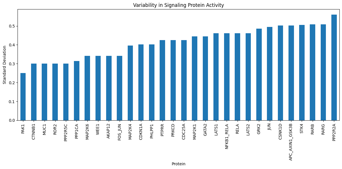
# Focus on signaling proteins with no measurement data
df_sig_prot_pred = df_vertex_val.loc[df_vertex_val.index.difference(dataset.data.query.pluck_features())]
df_sig_prot_pred.head()
| 0 | 1 | 2 | 3 | 4 | 5 | 6 | 7 | 8 | 9 | ... | 21 | 22 | 23 | 24 | 25 | 26 | 27 | 28 | 29 | 30 | |
|---|---|---|---|---|---|---|---|---|---|---|---|---|---|---|---|---|---|---|---|---|---|
| AAK1 | 0 | 0 | 0 | 0 | 0 | 0 | 0 | 0 | 0 | 0 | ... | 0 | 0 | 0 | 0 | 0 | 0 | 0 | 0 | 0 | 0 |
| ABI1 | 0 | 0 | 0 | 0 | 0 | 0 | 0 | 0 | 0 | 0 | ... | 0 | 0 | 0 | 0 | 0 | 0 | 0 | 0 | 0 | 0 |
| ABL1 | -1 | -1 | -1 | -1 | -1 | -1 | -1 | -1 | -1 | -1 | ... | -1 | -1 | -1 | -1 | -1 | -1 | -1 | -1 | -1 | -1 |
| ABL2 | 0 | 0 | 0 | 0 | 0 | 0 | 0 | 0 | 0 | 0 | ... | 0 | 0 | 0 | 0 | 0 | 0 | 0 | 0 | 0 | 0 |
| ABRAXAS1 | 0 | 0 | 0 | 0 | 0 | 0 | 0 | 0 | 0 | 0 | ... | 0 | 0 | 0 | 0 | 0 | 0 | 0 | 0 | 0 | 0 |
5 rows × 31 columns
# Visualize the variability in predicted signaling protein activities
import matplotlib.pyplot as plt

plt.figure(figsize=(12, 6))
df_sig_prot_pred.std(axis=1).sort_values().tail(30).plot.bar(title="Variability in Signaling Protein Activity")
plt.xlabel("Protein")
plt.ylabel("Standard Deviation")
plt.tight_layout()
plt.show()