Single sample intracellular signalling network inference#
In this notebook we showcase how to use the advanced CARNIVAL implementation available in CORNETO. This implementation extends the capabilities of the original CARNIVAL method by enabling advanced modelling and injection of knowledge for hypothesis generation. We will use a dataset consisting of 6 samples of hepatic stellate cells (HSC) where three of them were activated by the cytokine Transforming growth factor (TGF-β).
In the first part, we will show how to estimate Transcription Factor activities from gene expression data, following the Decoupler tutorial for functional analysis. Then, we will use the CARNIVAL method available in CORNETO to infer a network from TFs to receptors, assuming that we don’t really know which treatment was used. We will see how to do some basic modeling and adding information from pathway enrichment using PROGENy to bias the inferred networks.
NOTE: This tutorial uses the new Decoupler v2 version. We also use the highs solver, which has to be installed with
pip install highspy
import gzip
import os
import shutil
import tempfile
import urllib.request
import pandas as pd

# https://decoupler-py.readthedocs.io
import decoupler as dc
import numpy as np

# https://omnipathdb.org/
import omnipath as op

# Pydeseq for differential expression analysis
from pydeseq2.dds import DefaultInference, DeseqDataSet
from pydeseq2.ds import DeseqStats

# https://corneto.org
import corneto as cn
dc.__version__
'2.0.4'
max_time = 300
seed = 0
# Load the dataset
adata = dc.ds.hsctgfb()
adata
AnnData object with n_obs × n_vars = 6 × 58674
    obs: 'condition', 'sample_id'
Data preprocessing#
We will use AnnData and PyDeseq2 to pre-process the data and compute differential expression between control and tretament
# Obtain genes that pass the thresholds
dc.pp.filter_by_expr(
    adata=adata,
    group="condition",
    min_count=10,
    min_total_count=15,
    large_n=10,
    min_prop=0.7,
)
adata
AnnData object with n_obs × n_vars = 6 × 19510
    obs: 'condition', 'sample_id'
# Build DESeq2 object
inference = DefaultInference(n_cpus=8)
dds = DeseqDataSet(
    adata=adata,
    design_factors="condition",
    refit_cooks=True,
    inference=inference,
)

# Compute LFCs
dds.deseq2()

# Extract contrast between conditions
stat_res = DeseqStats(dds, contrast=["condition", "treatment", "control"], inference=inference)

# Compute Wald test
stat_res.summary()
Using None as control genes, passed at DeseqDataSet initialization
Log2 fold change & Wald test p-value: condition treatment vs control
                  baseMean  log2FoldChange     lfcSE       stat  \
RP11-347I19.8    88.877997       -0.207119  0.252510  -0.820242
TMEM170B        103.807801       -0.276960  0.210533  -1.315516
RP11-91P24.6    185.514929       -0.305844  0.180907  -1.690620
SLC33A1        2559.269047        0.595912  0.085251   6.990075
SNORA61          66.168502        0.746772  0.266416   2.803032
...                    ...             ...       ...        ...
RP11-75I2.3     771.828248        3.812419  0.128104  29.760449
SLC25A24       3525.523888        0.651017  0.087598   7.431841
BTN2A2          674.018191       -0.107905  0.106212  -1.015945
RP11-101E3.5    194.084339        0.092515  0.181943   0.508484
RP11-91I8.3      10.761886       -3.804522  0.920080  -4.134989

                      pvalue           padj
RP11-347I19.8   4.120781e-01   5.540360e-01
TMEM170B        1.883365e-01   3.052879e-01
RP11-91P24.6    9.090941e-02   1.681656e-01
SLC33A1         2.747400e-12   2.423226e-11
SNORA61         5.062459e-03   1.380028e-02
...                      ...            ...
RP11-75I2.3    1.270300e-194  4.130591e-192
SLC25A24        1.070963e-13   1.049974e-12
BTN2A2          3.096555e-01   4.491264e-01
RP11-101E3.5    6.111136e-01   7.290020e-01
RP11-91I8.3     3.549714e-05   1.471318e-04

[19510 rows x 6 columns]
results_df = stat_res.results_df
results_df
| baseMean | log2FoldChange | lfcSE | stat | pvalue | padj | |
|---|---|---|---|---|---|---|
| RP11-347I19.8 | 88.877997 | -0.207119 | 0.252510 | -0.820242 | 4.120781e-01 | 5.540360e-01 |
| TMEM170B | 103.807801 | -0.276960 | 0.210533 | -1.315516 | 1.883365e-01 | 3.052879e-01 |
| RP11-91P24.6 | 185.514929 | -0.305844 | 0.180907 | -1.690620 | 9.090941e-02 | 1.681656e-01 |
| SLC33A1 | 2559.269047 | 0.595912 | 0.085251 | 6.990075 | 2.747400e-12 | 2.423226e-11 |
| SNORA61 | 66.168502 | 0.746772 | 0.266416 | 2.803032 | 5.062459e-03 | 1.380028e-02 |
| ... | ... | ... | ... | ... | ... | ... |
| RP11-75I2.3 | 771.828248 | 3.812419 | 0.128104 | 29.760449 | 1.270300e-194 | 4.130591e-192 |
| SLC25A24 | 3525.523888 | 0.651017 | 0.087598 | 7.431841 | 1.070963e-13 | 1.049974e-12 |
| BTN2A2 | 674.018191 | -0.107905 | 0.106212 | -1.015945 | 3.096555e-01 | 4.491264e-01 |
| RP11-101E3.5 | 194.084339 | 0.092515 | 0.181943 | 0.508484 | 6.111136e-01 | 7.290020e-01 |
| RP11-91I8.3 | 10.761886 | -3.804522 | 0.920080 | -4.134989 | 3.549714e-05 | 1.471318e-04 |
19510 rows × 6 columns
data = results_df[["stat"]].T.rename(index={"stat": "treatment.vs.control"})
data
| RP11-347I19.8 | TMEM170B | RP11-91P24.6 | SLC33A1 | SNORA61 | THAP9-AS1 | LIX1L | TTC8 | WBSCR22 | LPHN2 | ... | STARD4-AS1 | ZNF845 | NIPSNAP3B | ARL6IP5 | MATN1-AS1 | RP11-75I2.3 | SLC25A24 | BTN2A2 | RP11-101E3.5 | RP11-91I8.3 | |
|---|---|---|---|---|---|---|---|---|---|---|---|---|---|---|---|---|---|---|---|---|---|
| treatment.vs.control | -0.820242 | -1.315516 | -1.69062 | 6.990075 | 2.803032 | 1.531275 | 2.164138 | -0.579879 | -0.945672 | -14.351588 | ... | 14.484214 | 0.56727 | -1.883272 | -8.42519 | -1.739921 | 29.760449 | 7.431841 | -1.015945 | 0.508484 | -4.134989 |
1 rows × 19510 columns
Prior knowledge with Decoupler and Omnipath#
# Retrieve CollecTRI gene regulatory network (through Omnipath).
# These are regulons that we will use for enrichment tests
# to infer TF activities
collectri = dc.op.collectri(organism="human")
collectri
| source | target | weight | resources | references | sign_decision | |
|---|---|---|---|---|---|---|
| 0 | MYC | TERT | 1.0 | DoRothEA-A;ExTRI;HTRI;NTNU.Curated;Pavlidis202... | 10022128;10491298;10606235;10637317;10723141;1... | PMID |
| 1 | SPI1 | BGLAP | 1.0 | ExTRI | 10022617 | default activation |
| 2 | SMAD3 | JUN | 1.0 | ExTRI;NTNU.Curated;TFactS;TRRUST | 10022869;12374795 | PMID |
| 3 | SMAD4 | JUN | 1.0 | ExTRI;NTNU.Curated;TFactS;TRRUST | 10022869;12374795 | PMID |
| 4 | STAT5A | IL2 | 1.0 | ExTRI | 10022878;11435608;17182565;17911616;22854263;2... | default activation |
| ... | ... | ... | ... | ... | ... | ... |
| 42985 | NFKB | hsa-miR-143-3p | 1.0 | ExTRI | 19472311 | default activation |
| 42986 | AP1 | hsa-miR-206 | 1.0 | ExTRI;GEREDB;NTNU.Curated | 19721712 | PMID |
| 42987 | NFKB | hsa-miR-21 | 1.0 | ExTRI | 20813833;22387281 | default activation |
| 42988 | NFKB | hsa-miR-224-5p | 1.0 | ExTRI | 23474441;23988648 | default activation |
| 42989 | AP1 | hsa-miR-144-3p | 1.0 | ExTRI | 23546882 | default activation |
42990 rows × 6 columns
# Run
tf_acts, tf_padj = dc.mt.ulm(data=data, net=collectri)

# Filter by sign padj
msk = (tf_padj.T < 0.05).iloc[:, 0]
tf_acts = tf_acts.loc[:, msk]

tf_acts
| APEX1 | ARID1A | ARID4B | ARNT | ASXL1 | ATF6 | BARX2 | BCL11A | BCL11B | BMAL2 | ... | TBX10 | TCF21 | TFAP2C | TP53 | VEZF1 | WWTR1 | ZBTB33 | ZEB2 | ZNF804A | ZXDC | |
|---|---|---|---|---|---|---|---|---|---|---|---|---|---|---|---|---|---|---|---|---|---|
| treatment.vs.control | -2.65907 | -3.917428 | -2.808733 | 3.174004 | 3.747021 | 2.707775 | 5.35855 | 2.649554 | -4.204618 | 3.869672 | ... | -3.705089 | 6.163829 | -2.579863 | -3.571649 | 4.208695 | -3.968034 | 3.238391 | 5.791132 | 3.366525 | -2.734602 |
1 rows × 143 columns
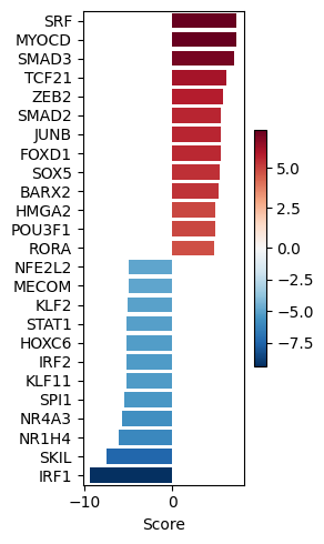
dc.pl.barplot(data=tf_acts, name="treatment.vs.control", top=25, figsize=(3, 5))
# We obtain ligand-receptor interactions from Omnipath, and we keep only the receptors
# This is our list of a prior potential receptors from which we will infer the network
unique_receptors = set(op.interactions.LigRecExtra.get(genesymbols=True)["target_genesymbol"].values.tolist())
len(unique_receptors)
1201
df_de_receptors = results_df.loc[results_df.index.intersection(unique_receptors)]
df_de_receptors = df_de_receptors[df_de_receptors.pvalue <= 1e-3]
df_de_receptors = df_de_receptors.sort_values(by="stat", ascending=False)
df_de_receptors
| baseMean | log2FoldChange | lfcSE | stat | pvalue | padj | |
|---|---|---|---|---|---|---|
| CDH6 | 28267.981856 | 3.020228 | 0.077434 | 39.003986 | 0.000000e+00 | 0.000000e+00 |
| CRLF1 | 7921.375581 | 3.342105 | 0.088004 | 37.976732 | 0.000000e+00 | 0.000000e+00 |
| FZD8 | 2720.368078 | 3.843472 | 0.102667 | 37.436438 | 9.984600e-307 | 1.025261e-303 |
| CDH2 | 7112.916583 | 2.809906 | 0.081906 | 34.306464 | 6.285559e-258 | 3.606802e-255 |
| DYSF | 441.551809 | 4.593718 | 0.182110 | 25.225001 | 2.130572e-140 | 3.711381e-138 |
| ... | ... | ... | ... | ... | ... | ... |
| TNFRSF1B | 646.930651 | -3.540723 | 0.137121 | -25.821870 | 5.038067e-147 | 9.542979e-145 |
| CHRM2 | 5807.106139 | -2.477402 | 0.086007 | -28.804799 | 1.867752e-182 | 5.521189e-180 |
| TNFRSF19 | 4210.866189 | -3.038970 | 0.101233 | -30.019698 | 5.430089e-198 | 1.858615e-195 |
| LPAR1 | 12716.045776 | -2.581318 | 0.070856 | -36.430237 | 1.414312e-290 | 1.103729e-287 |
| SMAD3 | 13965.722982 | -3.073656 | 0.072182 | -42.582053 | 0.000000e+00 | 0.000000e+00 |
283 rows × 6 columns
dc.pl.volcano(
    data=df_de_receptors,
    x="log2FoldChange",
    y="padj",
    top=20,
)
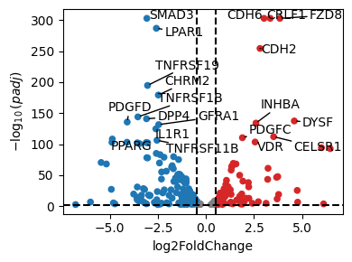
# We will take the top 20 receptors that increased the expression after treatment
df_top_receptors = df_de_receptors.head(20)
df_top_receptors
| baseMean | log2FoldChange | lfcSE | stat | pvalue | padj | |
|---|---|---|---|---|---|---|
| CDH6 | 28267.981856 | 3.020228 | 0.077434 | 39.003986 | 0.000000e+00 | 0.000000e+00 |
| CRLF1 | 7921.375581 | 3.342105 | 0.088004 | 37.976732 | 0.000000e+00 | 0.000000e+00 |
| FZD8 | 2720.368078 | 3.843472 | 0.102667 | 37.436438 | 9.984600e-307 | 1.025261e-303 |
| CDH2 | 7112.916583 | 2.809906 | 0.081906 | 34.306464 | 6.285559e-258 | 3.606802e-255 |
| DYSF | 441.551809 | 4.593718 | 0.182110 | 25.225001 | 2.130572e-140 | 3.711381e-138 |
| INHBA | 24333.979039 | 2.599031 | 0.104354 | 24.905991 | 6.407468e-137 | 1.041748e-134 |
| CELSR1 | 492.430456 | 3.517760 | 0.154404 | 22.782885 | 6.777783e-115 | 8.815637e-113 |
| PDGFC | 5482.100375 | 1.895284 | 0.083804 | 22.615764 | 3.032358e-113 | 3.917967e-111 |
| VDR | 1450.584956 | 2.555486 | 0.116713 | 21.895517 | 2.866339e-106 | 3.389228e-104 |
| HHIP | 379.147209 | 6.006281 | 0.287273 | 20.907896 | 4.538088e-97 | 4.426905e-95 |
| IGF1 | 361.270588 | 6.463104 | 0.311704 | 20.734725 | 1.684142e-95 | 1.595030e-93 |
| NPTN | 12642.896518 | 1.419111 | 0.079336 | 17.887451 | 1.477122e-71 | 9.062470e-70 |
| EFNB2 | 3320.622767 | 1.560757 | 0.087882 | 17.759772 | 1.448216e-70 | 8.640581e-69 |
| ITGB3 | 6531.344110 | 1.365175 | 0.078855 | 17.312493 | 3.786612e-67 | 2.069378e-65 |
| TGFB1 | 8949.673773 | 1.335719 | 0.077680 | 17.195118 | 2.888671e-66 | 1.552561e-64 |
| IL21R | 259.279854 | 3.228392 | 0.191940 | 16.819816 | 1.747011e-63 | 8.876088e-62 |
| ITGA1 | 26227.719647 | 1.310776 | 0.079834 | 16.418868 | 1.401577e-60 | 6.653227e-59 |
| FAP | 7232.349199 | 1.751321 | 0.115213 | 15.200707 | 3.498272e-52 | 1.392883e-50 |
| EGF | 144.293093 | 3.733752 | 0.251374 | 14.853364 | 6.616320e-50 | 2.458751e-48 |
| ITGA11 | 12473.737723 | 3.673720 | 0.250064 | 14.691129 | 7.347932e-49 | 2.630425e-47 |
Inferring intracellular signalling network with CARNIVAL and CORNETO#
CORNETO is a unified framework for knowledge-driven network inference. It includes a very flexible implementation of CARNIVAL that expands its original capabilities. We will see how to use it under different assumptions to extract a network from a prior knowledge network and a set of potential receptors + our estimated TFs
cn.info()

|
|
from corneto.methods.future import CarnivalFlow

CarnivalFlow.show_references()
- Pablo Rodriguez-Mier, Martin Garrido-Rodriguez, Attila Gabor, Julio Saez-Rodriguez. Unified knowledge-driven network inference from omics data. bioRxiv, pp. 10 (2024).
- Anika Liu, Panuwat Trairatphisan, Enio Gjerga, Athanasios Didangelos, Jonathan Barratt, Julio Saez-Rodriguez. From expression footprints to causal pathways: contextualizing large signaling networks with CARNIVAL. NPJ systems biology and applications, Vol. 5, No. 1, pp. 40 (2019).
# We get only interactions from SIGNOR http://signor.uniroma2.it/
pkn = op.interactions.OmniPath.get(databases=["SIGNOR"], genesymbols=True)
pkn = pkn[pkn.consensus_direction == True]
pkn.head()
| source | target | source_genesymbol | target_genesymbol | is_directed | is_stimulation | is_inhibition | consensus_direction | consensus_stimulation | consensus_inhibition | curation_effort | references | sources | n_sources | n_primary_sources | n_references | references_stripped | |
|---|---|---|---|---|---|---|---|---|---|---|---|---|---|---|---|---|---|
| 0 | Q13976 | Q13507 | PRKG1 | TRPC3 | True | False | True | True | False | True | 9 | HPRD:14983059;KEA:14983059;ProtMapper:14983059... | HPRD;HPRD_KEA;HPRD_MIMP;KEA;MIMP;PhosphoPoint;... | 15 | 8 | 2 | 14983059;16331690 |
| 1 | Q13976 | Q9HCX4 | PRKG1 | TRPC7 | True | True | False | True | True | False | 3 | SIGNOR:21402151;TRIP:21402151;iPTMnet:21402151 | SIGNOR;TRIP;iPTMnet | 3 | 3 | 1 | 21402151 |
| 2 | Q13438 | Q9HBA0 | OS9 | TRPV4 | True | True | True | True | True | True | 3 | HPRD:17932042;SIGNOR:17932042;TRIP:17932042 | HPRD;SIGNOR;TRIP | 3 | 3 | 1 | 17932042 |
| 3 | P18031 | Q9H1D0 | PTPN1 | TRPV6 | True | False | True | True | False | True | 11 | DEPOD:15894168;DEPOD:17197020;HPRD:15894168;In... | DEPOD;HPRD;IntAct;Lit-BM-17;SIGNOR;SPIKE_LC;TRIP | 7 | 6 | 2 | 15894168;17197020 |
| 4 | P63244 | Q9BX84 | RACK1 | TRPM6 | True | False | True | True | False | True | 2 | SIGNOR:18258429;TRIP:18258429 | SIGNOR;TRIP | 2 | 2 | 1 | 18258429 |
pkn["interaction"] = pkn["is_stimulation"].astype(int) - pkn["is_inhibition"].astype(int)
sel_pkn = pkn[["source_genesymbol", "interaction", "target_genesymbol"]]
sel_pkn
| source_genesymbol | interaction | target_genesymbol | |
|---|---|---|---|
| 0 | PRKG1 | -1 | TRPC3 |
| 1 | PRKG1 | 1 | TRPC7 |
| 2 | OS9 | 0 | TRPV4 |
| 3 | PTPN1 | -1 | TRPV6 |
| 4 | RACK1 | -1 | TRPM6 |
| ... | ... | ... | ... |
| 61542 | APC_PUF60_SIAH1_SKP1_TBL1X | -1 | CTNNB1 |
| 61543 | MAP2K6 | 1 | MAPK10 |
| 61544 | PRKAA1 | 1 | TP53 |
| 61545 | CNOT1_CNOT10_CNOT11_CNOT2_CNOT3_CNOT4_CNOT6_CN... | -1 | NANOS2 |
| 61546 | WNT16 | 1 | FZD3 |
60921 rows × 3 columns
# We create the CORNETO graph by importing the edges and interaction
from corneto.io import load_graph_from_sif_tuples

G = load_graph_from_sif_tuples([(r[0], r[1], r[2]) for _, r in sel_pkn.iterrows() if r[1] != 0])
G.shape
(5442, 60034)
# As measurements, we take the estimated TFs, we will filter out TFs with p-val > 0.001
significant_tfs = tf_acts[tf_padj <= 0.001].T.dropna().sort_values(by="treatment.vs.control", ascending=False)
significant_tfs
| treatment.vs.control | |
|---|---|
| SRF | 7.386495 |
| MYOCD | 7.347742 |
| SMAD3 | 7.088954 |
| TCF21 | 6.163829 |
| ZEB2 | 5.791132 |
| SMAD2 | 5.618762 |
| JUNB | 5.615222 |
| FOXD1 | 5.569866 |
| SOX5 | 5.389520 |
| BARX2 | 5.358550 |
| HMGA2 | 4.922228 |
| POU3F1 | 4.907625 |
| RORA | 4.752798 |
| SMAD4 | 4.444091 |
| OVOL1 | 4.283683 |
| MEF2A | 4.237091 |
| FGF2 | 4.210589 |
| VEZF1 | 4.208695 |
| SMAD5 | -4.006207 |
| CIITA | -4.135701 |
| NFKBIB | -4.156185 |
| REL | -4.166855 |
| PITX3 | -4.200417 |
| BCL11B | -4.204618 |
| IRF3 | -4.274769 |
| PITX1 | -4.343406 |
| PARK7 | -4.447971 |
| KLF8 | -4.469644 |
| DNMT3A | -4.642777 |
| RELB | -4.684388 |
| NFE2L2 | -4.912650 |
| MECOM | -4.945147 |
| KLF2 | -5.097029 |
| STAT1 | -5.190882 |
| HOXC6 | -5.261961 |
| IRF2 | -5.272425 |
| KLF11 | -5.272849 |
| SPI1 | -5.424463 |
| NR4A3 | -5.726818 |
| NR1H4 | -6.058745 |
| SKIL | -7.437972 |
| IRF1 | -9.363009 |
# We keep only the ones in the PKN graph
measurements = significant_tfs.loc[significant_tfs.index.intersection(G.V)].to_dict()["treatment.vs.control"]
measurements
{'SRF': 7.386495312851475,
 'MYOCD': 7.3477418488593,
 'SMAD3': 7.088953922116064,
 'ZEB2': 5.7911322785963435,
 'SMAD2': 5.618762357005816,
 'JUNB': 5.615222387859854,
 'HMGA2': 4.922227935739035,
 'POU3F1': 4.907624790924594,
 'RORA': 4.752798433353922,
 'SMAD4': 4.444090714736604,
 'MEF2A': 4.237091117534177,
 'FGF2': 4.210588858175027,
 'SMAD5': -4.006207147710557,
 'CIITA': -4.1357011230543845,
 'NFKBIB': -4.156185003186268,
 'REL': -4.1668552776199554,
 'PITX3': -4.20041706737378,
 'IRF3': -4.274768908592069,
 'PITX1': -4.3434055546060915,
 'KLF8': -4.469643880727271,
 'DNMT3A': -4.64277743087254,
 'RELB': -4.684387581686191,
 'NFE2L2': -4.912649636784848,
 'MECOM': -4.945146818217912,
 'STAT1': -5.190882487350966,
 'HOXC6': -5.261961030902404,
 'IRF2': -5.272425389933752,
 'KLF11': -5.272848781428293,
 'SPI1': -5.424462691953871,
 'NR4A3': -5.726818220249099,
 'NR1H4': -6.058745290814488,
 'SKIL': -7.437972448180294,
 'IRF1': -9.363009055573007}
# We will infer the direction, so for the inputs, we use a value of 0 (=unknown direction)
inputs = {k: 0 for k in df_top_receptors.index.intersection(G.V).values}
inputs
{'CDH6': 0,
 'CRLF1': 0,
 'FZD8': 0,
 'CDH2': 0,
 'INHBA': 0,
 'VDR': 0,
 'IGF1': 0,
 'EFNB2': 0,
 'ITGB3': 0,
 'TGFB1': 0,
 'IL21R': 0,
 'EGF': 0,
 'ITGA11': 0}
# Create the dataset in standard format
carnival_data = dict()
for inp, v in inputs.items():
    carnival_data[inp] = dict(value=v, role="input", mapping="vertex")
for out, v in measurements.items():
    carnival_data[out] = dict(value=v, role="output", mapping="vertex")
data = cn.Data.from_cdict({"sample1": carnival_data})
data
Data(n_samples=1, n_feats=[46])
CARNIVAL#
We will use now the standard CARNIVAL with a regularization penalty of 0.5. Typically, we would need additional data or information to select the optimal parameter. For hypothesis exploration, we can try different values and manually inspect the solutions
carnival = CarnivalFlow(lambda_reg=0.5)
P = carnival.build(G, data)
P.expr
Unreachable vertices for sample: 0
{'_flow': _flow: Variable((3279,), _flow),
 'edge_activates': edge_activates: Variable((3279, 1), edge_activates, boolean=True),
 'edge_inhibits': edge_inhibits: Variable((3279, 1), edge_inhibits, boolean=True),
 'const0x94da39a381f04fe': const0x94da39a381f04fe: Constant(CONSTANT, NONNEGATIVE, (947, 3279)),
 '_dag_layer': _dag_layer: Variable((947, 1), _dag_layer),
 'const0x1aa7a82deb9aa0b6': const0x1aa7a82deb9aa0b6: Constant(CONSTANT, NONNEGATIVE, (947, 3279)),
 'flow': _flow: Variable((3279,), _flow),
 'vertex_value': Expression(AFFINE, UNKNOWN, (947, 1)),
 'vertex_activated': Expression(AFFINE, NONNEGATIVE, (947, 1)),
 'vertex_inhibited': Expression(AFFINE, NONNEGATIVE, (947, 1)),
 'edge_value': Expression(AFFINE, UNKNOWN, (3279, 1)),
 'edge_has_signal': Expression(AFFINE, NONNEGATIVE, (3279, 1)),
 'vertex_max_depth': _dag_layer: Variable((947, 1), _dag_layer)}
P.solve(solver="highs", max_seconds=60, verbosity=1);
===============================================================================
                                     CVXPY
                                     v1.6.5
===============================================================================
(CVXPY) Jun 11 06:19:10 PM: Your problem has 10784 variables, 30852 constraints, and 1 parameters.
(CVXPY) Jun 11 06:19:10 PM: It is compliant with the following grammars: DCP, DQCP
(CVXPY) Jun 11 06:19:10 PM: CVXPY will first compile your problem; then, it will invoke a numerical solver to obtain a solution.
(CVXPY) Jun 11 06:19:10 PM: Your problem is compiled with the CPP canonicalization backend.
-------------------------------------------------------------------------------
                                  Compilation
-------------------------------------------------------------------------------
(CVXPY) Jun 11 06:19:10 PM: Compiling problem (target solver=HIGHS).
(CVXPY) Jun 11 06:19:10 PM: Reduction chain: Dcp2Cone -> CvxAttr2Constr -> ConeMatrixStuffing -> HIGHS
(CVXPY) Jun 11 06:19:10 PM: Applying reduction Dcp2Cone
(CVXPY) Jun 11 06:19:10 PM: Applying reduction CvxAttr2Constr
(CVXPY) Jun 11 06:19:10 PM: Applying reduction ConeMatrixStuffing
(CVXPY) Jun 11 06:19:10 PM: Applying reduction HIGHS
(CVXPY) Jun 11 06:19:10 PM: Finished problem compilation (took 6.457e-02 seconds).
(CVXPY) Jun 11 06:19:10 PM: (Subsequent compilations of this problem, using the same arguments, should take less time.)
-------------------------------------------------------------------------------
                                Numerical solver
-------------------------------------------------------------------------------
(CVXPY) Jun 11 06:19:10 PM: Invoking solver HIGHS  to obtain a solution.
Running HiGHS 1.11.0 (git hash: 364c83a): Copyright (c) 2025 HiGHS under MIT licence terms
MIP  has 30852 rows; 10784 cols; 108719 nonzeros; 6558 integer variables (6558 binary)
Coefficient ranges:
  Matrix [1e+00, 9e+02]
  Cost   [5e-01, 8e+00]
  Bound  [1e+00, 1e+00]
  RHS    [1e+00, 1e+03]
Presolving model
17921 rows, 10381 cols, 91785 nonzeros  0s
13133 rows, 9253 cols, 70701 nonzeros  0s
12754 rows, 9174 cols, 70260 nonzeros  0s

Solving MIP model with:
   12754 rows
   9174 cols (5768 binary, 0 integer, 0 implied int., 3406 continuous, 0 domain fixed)
   70260 nonzeros

Src: B => Branching; C => Central rounding; F => Feasibility pump; J => Feasibility jump;
     H => Heuristic; L => Sub-MIP; P => Empty MIP; R => Randomized rounding; Z => ZI Round;
     I => Shifting; S => Solve LP; T => Evaluate node; U => Unbounded; X => User solution;
     z => Trivial zero; l => Trivial lower; u => Trivial upper; p => Trivial point

        Nodes      |    B&B Tree     |            Objective Bounds              |  Dynamic Constraints |       Work
Src  Proc. InQueue |  Leaves   Expl. | BestBound       BestSol              Gap |   Cuts   InLp Confl. | LpIters     Time

 J       0       0         0   0.00%   -inf            0                  Large        0      0      0         0     0.4s
         0       0         0   0.00%   -100.0153165    0                  Large        0      0      0      1834     0.5s
 L       0       0         0   0.00%   -97.38159462    -90.88159462       7.15%     1663     70      0      3162     4.0s

1.5% inactive integer columns, restarting
Model after restart has 12621 rows, 9052 cols (5650 bin., 0 int., 0 impl., 3402 cont., 0 dom.fix.), and 69099 nonzeros

         0       0         0   0.00%   -97.38159462    -90.88159462       7.15%       27      0      0     12413     6.0s
         0       0         0   0.00%   -97.38159462    -90.88159462       7.15%       27     19     21     13585     6.1s
 L       0       0         0   0.00%   -97.38159462    -96.88159462       0.52%      365     58     21     13760     8.1s

11.6% inactive integer columns, restarting
Model after restart has 10990 rows, 8004 cols (4780 bin., 0 int., 0 impl., 3224 cont., 0 dom.fix.), and 57133 nonzeros

         0       0         0   0.00%   -97.38159462    -96.88159462       0.52%       27      0      0     18245     8.3s
         0       0         0   0.00%   -97.38159462    -96.88159462       0.52%       27     16      5     19546     8.3s

Symmetry detection completed in 0.0s
Found 19 generator(s)

        34       1        16  46.09%   -97.38159462    -96.88159462       0.52%      603     27   1383     43341    13.5s

Restarting search from the root node
Model after restart has 869 rows, 2591 cols (75 bin., 0 int., 0 impl., 2516 cont., 0 dom.fix.), and 6771 nonzeros

        50       0         0   0.00%   -97.37842673    -96.88159462       0.51%       10      0      0     55711    16.4s
        51       0         1 100.00%   -96.88159462    -96.88159462       0.00%       10      0      0     56356    16.4s

Solving report
  Status            Optimal
  Primal bound      -96.8815946237
  Dual bound        -96.8815946237
  Gap               0% (tolerance: 0.01%)
  P-D integral      0.338566345924
  Solution status   feasible
                    -96.8815946237 (objective)
                    0 (bound viol.)
                    2.22044604925e-16 (int. viol.)
                    0 (row viol.)
  Timing            16.42 (total)
                    0.00 (presolve)
                    0.00 (solve)
                    0.00 (postsolve)
  Max sub-MIP depth 8
  Nodes             51
  Repair LPs        0 (0 feasible; 0 iterations)
  LP iterations     56356 (total)
                    28833 (strong br.)
                    1751 (separation)
                    13653 (heuristics)
-------------------------------------------------------------------------------
                                    Summary
-------------------------------------------------------------------------------
(CVXPY) Jun 11 06:19:27 PM: Problem status: optimal
(CVXPY) Jun 11 06:19:27 PM: Optimal value: 2.650e+01
(CVXPY) Jun 11 06:19:27 PM: Compilation took 6.457e-02 seconds
(CVXPY) Jun 11 06:19:27 PM: Solver (including time spent in interface) took 1.643e+01 seconds
# Error for sample is 0, meaning that all reachable TFs (from receptors) are correctly explained
for o in P.objectives:
    print(o.name, "->", o.value)
error_sample1_0 -> 1.050898412285121e-15
regularization_edge_has_signal -> 53.0
# We extract the selected edges
sol_edges = np.flatnonzero(np.abs(P.expr.edge_value.value) > 0.5)
carnival.processed_graph.plot_values(
    vertex_values=P.expr.vertex_value.value,
    edge_values=P.expr.edge_value.value,
    edge_indexes=sol_edges,
)

# Extracting the solution graph
G_sol = carnival.processed_graph.edge_subgraph(sol_edges)
G_sol.shape
(53, 53)
pd.DataFrame(
    P.expr.vertex_value.value,
    index=carnival.processed_graph.V,
    columns=["node_activity"],
)
| node_activity | |
|---|---|
| PTPRC | 0.0 |
| GEM | 0.0 |
| MYO10 | 0.0 |
| ARHGEF12 | 0.0 |
| TP53RK | 0.0 |
| ... | ... |
| NUAK1 | 0.0 |
| CAMKK2 | 0.0 |
| P0C725_UBB | 0.0 |
| CSNK2B | 0.0 |
| ANAPC1_ANAPC10_ANAPC11_ANAPC13_ANAPC2_ANAPC4_ANAPC5_ANAPC7_CDC16_CDC23_CDC26_CDC27 | 0.0 |
947 rows × 1 columns
pd.DataFrame(P.expr.edge_value.value, index=carnival.processed_graph.E, columns=["edge_activity"])
| edge_activity | ||
|---|---|---|
| (SMAD3) | (MYOD1) | 0.0 |
| (GRK2) | (BDKRB2) | 0.0 |
| (MAPK14) | (MAPKAPK2) | 0.0 |
| (DEPTOR_EEF1A1_MLST8_MTOR_PRR5_RICTOR) | (FBXW8) | 0.0 |
| (SLK) | (MAP3K5) | 0.0 |
| ... | ... | ... |
| () | (FZD8) | 0.0 |
| (IL21R) | 0.0 | |
| (EGF) | 0.0 | |
| (TGFB1) | 0.0 | |
| (CDH2) | 0.0 |
3279 rows × 1 columns
Changing modelling assumptions#
Thanks to CORNETO’s modeling capabilities, we can manipulate the problems to add more knowledge, new objectives or different constraints. As an example, we are going to penalize the use of inhibitory interactions from the PKN to simplify the reconstructed networks in CARNIVAL
edge_interactions = np.array(carnival.processed_graph.get_attr_from_edges("interaction"))
penalties = np.zeros_like(edge_interactions)
# We add a large penalty to each interaction which is inhibitory (-1)
penalties[edge_interactions == -1] = 10
penalties.shape
(3279,)
# We use the edge_has_signal variable (1 if selected to propagate signal, 0 otherwise),
# and we multiply with  the penalties
(P.expr.edge_has_signal.T @ penalties).shape
(1,)
P.add_objectives(P.expr.edge_has_signal.T @ penalties)
P.solve(solver="highs", max_seconds=60, verbosity=1);
===============================================================================
                                     CVXPY
                                     v1.6.5
===============================================================================
(CVXPY) Jun 11 06:19:27 PM: Your problem has 10784 variables, 30852 constraints, and 1 parameters.
(CVXPY) Jun 11 06:19:27 PM: It is compliant with the following grammars: DCP, DQCP
(CVXPY) Jun 11 06:19:27 PM: CVXPY will first compile your problem; then, it will invoke a numerical solver to obtain a solution.
(CVXPY) Jun 11 06:19:27 PM: Your problem is compiled with the CPP canonicalization backend.
-------------------------------------------------------------------------------
                                  Compilation
-------------------------------------------------------------------------------
(CVXPY) Jun 11 06:19:27 PM: Compiling problem (target solver=HIGHS).
(CVXPY) Jun 11 06:19:27 PM: Reduction chain: Dcp2Cone -> CvxAttr2Constr -> ConeMatrixStuffing -> HIGHS
(CVXPY) Jun 11 06:19:27 PM: Applying reduction Dcp2Cone
(CVXPY) Jun 11 06:19:27 PM: Applying reduction CvxAttr2Constr
(CVXPY) Jun 11 06:19:27 PM: Applying reduction ConeMatrixStuffing
(CVXPY) Jun 11 06:19:27 PM: Applying reduction HIGHS
(CVXPY) Jun 11 06:19:27 PM: Finished problem compilation (took 5.865e-02 seconds).
(CVXPY) Jun 11 06:19:27 PM: (Subsequent compilations of this problem, using the same arguments, should take less time.)
-------------------------------------------------------------------------------
                                Numerical solver
-------------------------------------------------------------------------------
(CVXPY) Jun 11 06:19:27 PM: Invoking solver HIGHS  to obtain a solution.
Running HiGHS 1.11.0 (git hash: 364c83a): Copyright (c) 2025 HiGHS under MIT licence terms
MIP  has 30852 rows; 10784 cols; 108719 nonzeros; 6558 integer variables (6558 binary)
Coefficient ranges:
  Matrix [1e+00, 9e+02]
  Cost   [5e-01, 2e+01]
  Bound  [1e+00, 1e+00]
  RHS    [1e+00, 1e+03]
Presolving model
17921 rows, 10381 cols, 91785 nonzeros  0s
13026 rows, 9212 cols, 70234 nonzeros  0s
12645 rows, 9131 cols, 69798 nonzeros  0s

Solving MIP model with:
   12645 rows
   9131 cols (5727 binary, 0 integer, 0 implied int., 3404 continuous, 0 domain fixed)
   69798 nonzeros

Src: B => Branching; C => Central rounding; F => Feasibility pump; J => Feasibility jump;
     H => Heuristic; L => Sub-MIP; P => Empty MIP; R => Randomized rounding; Z => ZI Round;
     I => Shifting; S => Solve LP; T => Evaluate node; U => Unbounded; X => User solution;
     z => Trivial zero; l => Trivial lower; u => Trivial upper; p => Trivial point

        Nodes      |    B&B Tree     |            Objective Bounds              |  Dynamic Constraints |       Work
Src  Proc. InQueue |  Leaves   Expl. | BestBound       BestSol              Gap |   Cuts   InLp Confl. | LpIters     Time

 J       0       0         0   0.00%   -inf            0                  Large        0      0      0         0     0.4s
         0       0         0   0.00%   -80.01008213    0                  Large        0      0      0      1331     0.5s
 C       0       0         0   0.00%   -72.82817579    -2.006207148    3530.14%      356     21      0      1844     1.2s
 L       0       0         0   0.00%   -72.41150912    -72.41150912       0.00%     1082     50      0      2307     2.5s
         1       0         1 100.00%   -72.41150912    -72.41150912       0.00%     1082     50      0      4414     2.5s

Solving report
  Status            Optimal
  Primal bound      -72.411509124
  Dual bound        -72.411509124
  Gap               0% (tolerance: 0.01%)
  P-D integral      46.7809634959
  Solution status   feasible
                    -72.411509124 (objective)
                    0 (bound viol.)
                    0 (int. viol.)
                    0 (row viol.)
  Timing            2.53 (total)
                    0.00 (presolve)
                    0.00 (solve)
                    0.00 (postsolve)
  Max sub-MIP depth 5
  Nodes             1
  Repair LPs        0 (0 feasible; 0 iterations)
  LP iterations     4414 (total)
                    0 (strong br.)
                    976 (separation)
                    2107 (heuristics)
-------------------------------------------------------------------------------
                                    Summary
-------------------------------------------------------------------------------
(CVXPY) Jun 11 06:19:30 PM: Problem status: optimal
(CVXPY) Jun 11 06:19:30 PM: Optimal value: 5.097e+01
(CVXPY) Jun 11 06:19:30 PM: Compilation took 5.865e-02 seconds
(CVXPY) Jun 11 06:19:30 PM: Solver (including time spent in interface) took 2.544e+00 seconds
# Note that the networks have a larger error (many TFs are now not explained)
for o in P.objectives:
    print(o.value)
26.970085499734868
48.0
[0.]
# We extract the selected edges. Networks are simpler,
# and they show again some activation of CDH2 and inhibition of IGF1
sol_edges = np.flatnonzero(np.abs(P.expr.edge_value.value) > 0.5)
carnival.processed_graph.plot_values(
    vertex_values=P.expr.vertex_value.value,
    edge_values=P.expr.edge_value.value,
    edge_indexes=sol_edges,
)

Other options#
We included an option to simplify the networks inferred by CARNIVAL, by penalizing the selection of indirect rules. These rules are:
A -> B in the PKN, and we observe B is downregulated, we explain it with downregulation of its upstream gene A
A -| B in the PKN, and we observe B is upregulated, we explain it with downregulation of A
NOTE: This is an experimental feature and was not benchmarked in the original CARNIVAL paper.
carnival = CarnivalFlow(lambda_reg=0.5, indirect_rule_penalty=10)
P = carnival.build(G, data)
P.expr
Unreachable vertices for sample: 0
{'_flow': _flow: Variable((3279,), _flow),
 'edge_inhibits': edge_inhibits: Variable((3279, 1), edge_inhibits, boolean=True),
 'edge_activates': edge_activates: Variable((3279, 1), edge_activates, boolean=True),
 'const0x1735def7420c5858': const0x1735def7420c5858: Constant(CONSTANT, NONNEGATIVE, (947, 3279)),
 '_dag_layer': _dag_layer: Variable((947, 1), _dag_layer),
 'const0xb46ccbceabe3b17': const0xb46ccbceabe3b17: Constant(CONSTANT, NONNEGATIVE, (947, 3279)),
 'flow': _flow: Variable((3279,), _flow),
 'vertex_value': Expression(AFFINE, UNKNOWN, (947, 1)),
 'vertex_activated': Expression(AFFINE, NONNEGATIVE, (947, 1)),
 'vertex_inhibited': Expression(AFFINE, NONNEGATIVE, (947, 1)),
 'edge_value': Expression(AFFINE, UNKNOWN, (3279, 1)),
 'edge_has_signal': Expression(AFFINE, NONNEGATIVE, (3279, 1)),
 'vertex_max_depth': _dag_layer: Variable((947, 1), _dag_layer)}
P.solve(solver="highs", max_seconds=60, verbosity=1);
===============================================================================
                                     CVXPY
                                     v1.6.5
===============================================================================
(CVXPY) Jun 11 06:19:30 PM: Your problem has 10784 variables, 30852 constraints, and 1 parameters.
(CVXPY) Jun 11 06:19:30 PM: It is compliant with the following grammars: DCP, DQCP
(CVXPY) Jun 11 06:19:30 PM: CVXPY will first compile your problem; then, it will invoke a numerical solver to obtain a solution.
(CVXPY) Jun 11 06:19:30 PM: Your problem is compiled with the CPP canonicalization backend.
-------------------------------------------------------------------------------
                                  Compilation
-------------------------------------------------------------------------------
(CVXPY) Jun 11 06:19:30 PM: Compiling problem (target solver=HIGHS).
(CVXPY) Jun 11 06:19:30 PM: Reduction chain: Dcp2Cone -> CvxAttr2Constr -> ConeMatrixStuffing -> HIGHS
(CVXPY) Jun 11 06:19:30 PM: Applying reduction Dcp2Cone
(CVXPY) Jun 11 06:19:30 PM: Applying reduction CvxAttr2Constr
(CVXPY) Jun 11 06:19:30 PM: Applying reduction ConeMatrixStuffing
(CVXPY) Jun 11 06:19:30 PM: Applying reduction HIGHS
(CVXPY) Jun 11 06:19:30 PM: Finished problem compilation (took 7.756e-02 seconds).
(CVXPY) Jun 11 06:19:30 PM: (Subsequent compilations of this problem, using the same arguments, should take less time.)
-------------------------------------------------------------------------------
                                Numerical solver
-------------------------------------------------------------------------------
(CVXPY) Jun 11 06:19:30 PM: Invoking solver HIGHS  to obtain a solution.
Running HiGHS 1.11.0 (git hash: 364c83a): Copyright (c) 2025 HiGHS under MIT licence terms
MIP  has 30852 rows; 10784 cols; 108719 nonzeros; 6558 integer variables (6558 binary)
Coefficient ranges:
  Matrix [1e+00, 9e+02]
  Cost   [5e-01, 2e+01]
  Bound  [1e+00, 1e+00]
  RHS    [1e+00, 1e+03]
Presolving model
17921 rows, 10381 cols, 91785 nonzeros  0s
12937 rows, 9173 cols, 69770 nonzeros  0s
12555 rows, 9092 cols, 69332 nonzeros  0s

Solving MIP model with:
   12555 rows
   9092 cols (5685 binary, 0 integer, 0 implied int., 3407 continuous, 0 domain fixed)
   69332 nonzeros

Src: B => Branching; C => Central rounding; F => Feasibility pump; J => Feasibility jump;
     H => Heuristic; L => Sub-MIP; P => Empty MIP; R => Randomized rounding; Z => ZI Round;
     I => Shifting; S => Solve LP; T => Evaluate node; U => Unbounded; X => User solution;
     z => Trivial zero; l => Trivial lower; u => Trivial upper; p => Trivial point

        Nodes      |    B&B Tree     |            Objective Bounds              |  Dynamic Constraints |       Work
Src  Proc. InQueue |  Leaves   Expl. | BestBound       BestSol              Gap |   Cuts   InLp Confl. | LpIters     Time

 J       0       0         0   0.00%   -inf            0                  Large        0      0      0         0     0.4s
         0       0         0   0.00%   -54.39752097    0                  Large        0      0     16       912     0.5s
 L       0       0         0   0.00%   -49.48644796    -48.98644796       1.02%      896     48     35      1408     3.0s

62.0% inactive integer columns, restarting
Model after restart has 4380 rows, 4101 cols (1192 bin., 0 int., 0 impl., 2909 cont., 0 dom.fix.), and 18621 nonzeros

         0       0         0   0.00%   -49.48644796    -48.98644796       1.02%       16      0      0      6197     3.4s
         0       0         0   0.00%   -49.48644796    -48.98644796       1.02%       16     13      7      6871     3.5s

Symmetry detection completed in 0.0s
Found 10 generator(s)

         5       0         3 100.00%   -48.98644796    -48.98644796       0.00%      726     19     46     13939     4.5s

Solving report
  Status            Optimal
  Primal bound      -48.9864479649
  Dual bound        -48.9864479649
  Gap               0% (tolerance: 0.01%)
  P-D integral      0.0145504962008
  Solution status   feasible
                    -48.9864479649 (objective)
                    0 (bound viol.)
                    0 (int. viol.)
                    0 (row viol.)
  Timing            4.46 (total)
                    0.00 (presolve)
                    0.00 (solve)
                    0.00 (postsolve)
  Max sub-MIP depth 5
  Nodes             5
  Repair LPs        0 (0 feasible; 0 iterations)
  LP iterations     13939 (total)
                    771 (strong br.)
                    770 (separation)
                    10556 (heuristics)
-------------------------------------------------------------------------------
                                    Summary
-------------------------------------------------------------------------------
(CVXPY) Jun 11 06:19:35 PM: Problem status: optimal
(CVXPY) Jun 11 06:19:35 PM: Optimal value: 7.440e+01
(CVXPY) Jun 11 06:19:35 PM: Compilation took 7.756e-02 seconds
(CVXPY) Jun 11 06:19:35 PM: Solver (including time spent in interface) took 4.473e+00 seconds
sol_edges = np.flatnonzero(np.abs(P.expr.edge_value.value) > 0.5)
carnival.processed_graph.plot_values(
    vertex_values=P.expr.vertex_value.value,
    edge_values=P.expr.edge_value.value,
    edge_indexes=sol_edges,
)

Using information from PROGENy#
In the previous examples, we used only information from TF activities and de-regulated receptors, and we tested different options. However, results can be highly variable, due to uncertainty in the intermediate signalling proteins (downstream receptors and upstream TFs), and due to the existence of multiple paths in the PKN.
Additional information can be used to bias the reconstruction towards more plausible signalling pathways. Here, we will use information from PROGENy, which infers pathway activities from gene expression data.
progeny = dc.op.progeny(organism="human")
progeny
| source | target | weight | padj | |
|---|---|---|---|---|
| 0 | Androgen | TMPRSS2 | 11.490631 | 2.384806e-47 |
| 1 | Androgen | NKX3-1 | 10.622551 | 2.205102e-44 |
| 2 | Androgen | MBOAT2 | 10.472733 | 4.632376e-44 |
| 3 | Androgen | KLK2 | 10.176186 | 1.944410e-40 |
| 4 | Androgen | SARG | 11.386852 | 2.790210e-40 |
| ... | ... | ... | ... | ... |
| 62456 | p53 | ENPP2 | 2.771405 | 4.993215e-02 |
| 62457 | p53 | ARRDC4 | 3.494328 | 4.996747e-02 |
| 62458 | p53 | MYO1B | -1.148057 | 4.997905e-02 |
| 62459 | p53 | CTSC | -1.784693 | 4.998864e-02 |
| 62460 | p53 | NAA50 | -1.435013 | 4.998884e-02 |
62461 rows × 4 columns
# We will use the PyDeseq2 stat as the score for the genes
de_data = results_df[["stat"]].T.rename(index={"stat": "treatment.vs.control"})
de_data
| RP11-347I19.8 | TMEM170B | RP11-91P24.6 | SLC33A1 | SNORA61 | THAP9-AS1 | LIX1L | TTC8 | WBSCR22 | LPHN2 | ... | STARD4-AS1 | ZNF845 | NIPSNAP3B | ARL6IP5 | MATN1-AS1 | RP11-75I2.3 | SLC25A24 | BTN2A2 | RP11-101E3.5 | RP11-91I8.3 | |
|---|---|---|---|---|---|---|---|---|---|---|---|---|---|---|---|---|---|---|---|---|---|
| treatment.vs.control | -0.820242 | -1.315516 | -1.69062 | 6.990075 | 2.803032 | 1.531275 | 2.164138 | -0.579879 | -0.945672 | -14.351588 | ... | 14.484214 | 0.56727 | -1.883272 | -8.42519 | -1.739921 | 29.760449 | 7.431841 | -1.015945 | 0.508484 | -4.134989 |
1 rows × 19510 columns
# Run
pw_acts, pw_padj = dc.mt.ulm(data=de_data, net=progeny)

# Filter by sign padj
msk = (pw_padj.T < 0.05).iloc[:, 0]
pw_acts = pw_acts.loc[:, msk]

pw_acts
| Androgen | EGFR | Estrogen | Hypoxia | JAK-STAT | MAPK | NFkB | PI3K | TGFb | TNFa | VEGF | p53 | |
|---|---|---|---|---|---|---|---|---|---|---|---|---|
| treatment.vs.control | 4.784375 | 17.220881 | 11.01434 | 5.69894 | -14.308169 | 25.560896 | -10.195328 | 24.644391 | 59.32932 | -9.129273 | 11.437564 | -12.589745 |
dc.pl.barplot(data=pw_acts, name="treatment.vs.control", top=25, figsize=(3, 3))
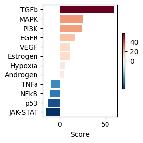
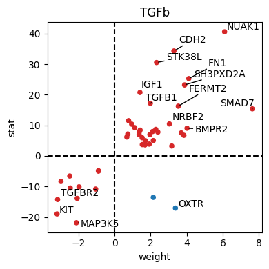
We can see that the TGFb pathway is predicted to be stimulated, using the observed downstream changes in gene expression. Now that we have this info, we can bias the networks towards the selection of signalling proteins in that pathway. We can check first the up/down genes in that pathway using the PROGENy network:
dc.pl.source_targets(data=results_df, x="weight", y="stat", net=progeny, name="TGFb", top=15, figsize=(4, 4))
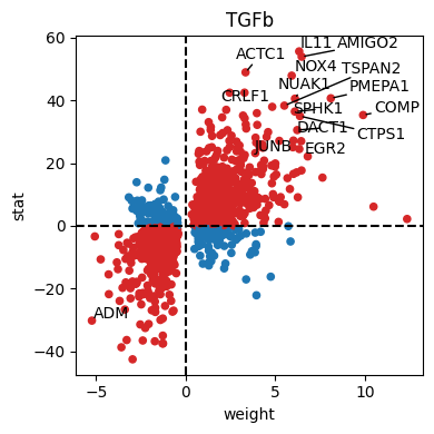
df_progeny_with_de = progeny[(progeny.source == "TGFb")].set_index("target").join(results_df, rsuffix="_deseq")
df_progeny_with_de = df_progeny_with_de[(df_progeny_with_de.padj_deseq <= 1e-2) & (df_progeny_with_de.padj <= 1e-2)]

# We remove the TFs, we keep only unscored nodes in the network
df_progeny_with_de = df_progeny_with_de.loc[df_progeny_with_de.index.difference(tf_acts.columns)]
# We will calculate an score of importance, based on the weight from progeny PKN (the coefficient of importance)
# and the stat from DESeq2 for that gene in our dataset
df_progeny_with_de["score"] = df_progeny_with_de["weight"].abs() * df_progeny_with_de["stat"].abs()
df_progeny_with_de
| source | weight | padj | baseMean | log2FoldChange | lfcSE | stat | pvalue | padj_deseq | score | |
|---|---|---|---|---|---|---|---|---|---|---|
| ABCA6 | TGFb | -3.271537 | 3.259776e-08 | 21.312146 | -3.113671 | 0.577035 | -5.395978 | 6.815130e-08 | 4.058705e-07 | 17.653141 |
| ABCA8 | TGFb | -1.709245 | 9.264710e-08 | 1241.936380 | -2.025544 | 0.110001 | -18.413859 | 1.017102e-75 | 6.681365e-74 | 31.473798 |
| ABL1 | TGFb | 1.417354 | 6.789650e-03 | 11992.405040 | 0.654017 | 0.077665 | 8.421013 | 3.732418e-17 | 4.470195e-16 | 11.935557 |
| ACOX1 | TGFb | 1.248375 | 1.198791e-04 | 1932.465662 | 0.501733 | 0.090449 | 5.547157 | 2.903517e-08 | 1.797196e-07 | 6.924934 |
| ACOX3 | TGFb | 2.721529 | 3.738116e-09 | 1298.226294 | 1.249147 | 0.089501 | 13.956818 | 2.859170e-44 | 9.070311e-43 | 37.983882 |
| ... | ... | ... | ... | ... | ... | ... | ... | ... | ... | ... |
| ZMIZ1 | TGFb | 1.957381 | 6.461094e-05 | 7721.447043 | 0.596702 | 0.085546 | 6.975202 | 3.054313e-12 | 2.685428e-11 | 13.653126 |
| ZNF281 | TGFb | 1.989687 | 3.593457e-04 | 2098.460557 | 0.586130 | 0.094963 | 6.172166 | 6.736069e-10 | 4.833421e-09 | 12.280681 |
| ZNF365 | TGFb | 1.237670 | 4.895429e-03 | 719.298471 | 2.121362 | 0.124407 | 17.051793 | 3.389758e-65 | 1.797124e-63 | 21.104492 |
| ZNF48 | TGFb | 1.745462 | 1.500992e-05 | 638.023400 | 0.728684 | 0.105677 | 6.895368 | 5.372537e-12 | 4.650319e-11 | 12.035601 |
| ZNF592 | TGFb | 0.740719 | 5.914911e-03 | 1654.348595 | 0.258427 | 0.088101 | 2.933306 | 3.353729e-03 | 9.545039e-03 | 2.172756 |
600 rows × 10 columns
# We will favor now the inclusion of these genes. We will
# increase lambda to get smaller networks for interpretation, and
# we will use a large penalty for indirect rules.
carnival = CarnivalFlow(lambda_reg=1.5, indirect_rule_penalty=1)
P = carnival.build(G, data)
Unreachable vertices for sample: 0
# We need to select the subset of genes in the processed graph, since after building carnival using the
# inputs (receptors) and TFs, the processed graph is pruned (unreachable genes removed) and thus many
# of the genes we want to score are not anymore in the graph
tgfb_genes = df_progeny_with_de.index.intersection(carnival.processed_graph.V).tolist()
len(tgfb_genes)
45
# We can visualize only the genes in the pruned PKN that carnival will use
# NOTE: The processed graph is the pruned PKN containing all interactions
# connecting the selected receptors to TFs, before inferring the signalling
# networks
dc.pl.source_targets(
    data=results_df.loc[tgfb_genes], x="weight", y="stat", net=progeny, name="TGFb", top=15, figsize=(4, 4)
)
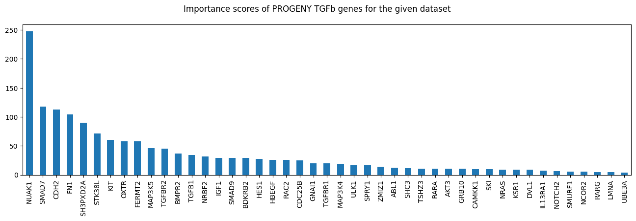
import matplotlib.pyplot as plt

fig, ax = plt.subplots(figsize=(16, 4))
df_progeny_with_de.loc[tgfb_genes, "score"].sort_values(ascending=False).plot.bar(ax=ax)
fig.suptitle("Importance scores of PROGENY TGFb genes for the given dataset");
# Scale factor for influence in the overall CARNIVAL obj function
influence_factor = 0.1

# Create the custom obj function to include in CARNIVAL
vertex_scores = np.zeros(len(carnival.processed_graph.V))
vertex_selected_var = P.expr.vertex_activated + P.expr.vertex_inhibited
for i, v in enumerate(carnival.processed_graph.V):
    if v in tgfb_genes:
        score = df_progeny_with_de.loc[v].score
        vertex_scores[i] = score
        print(i, v, score)

# The objective is just c^T @ penalties
obj = vertex_selected_var.T @ vertex_scores

# We add a negative weight to maximize selection
P.add_objective(obj, name="progeny_genes_score", weight=-influence_factor)
P.solve(solver="highs", max_seconds=60, verbosity=1);
21 NRAS 9.055651210075709
25 GNAI1 19.972682422333143
27 RAC2 25.75672169584716
44 STK38L 71.06848321367565
84 TGFBR1 19.78318967446914
101 CDH2 112.81029585047202
126 MAP3K4 18.633117866454263
148 SMURF1 5.687767369319471
189 SMAD9 29.108495622484853
208 CAMKK1 9.853578482249983
224 KIT 60.51896993721089
287 RARA 10.473371785649258
288 ULK1 16.78905409561297
295 HES1 27.774456156272613
314 UBE3A 4.198015442492376
324 SH3PXD2A 90.03028888776223
327 NOTCH2 6.0877870556111855
335 IGF1 29.197953109742727
370 NCOR2 5.253273919130532
412 ZMIZ1 13.653126134909561
434 RARG 4.459674733843175
438 IL13RA1 7.412771495771951
470 SPRY1 16.340142523123966
480 TSHZ3 10.746459209540498
533 HBEGF 25.871592750755017
538 LMNA 4.330586475862753
556 CDC25B 24.899175740820784
608 SHC3 11.348956411416047
643 DVL1 8.484789724643731
672 NRBF2 31.751626499871815
700 FN1 103.98952712958402
715 SMAD7 117.45746080491878
730 TGFBR2 45.037266815474084
749 SKI 9.483452356595494
758 GRB10 10.21623996260473
828 BDKRB2 28.78488734209394
881 AKT3 10.323123896941524
883 TGFB1 34.09092982693877
885 MAP3K5 46.20501733040189
919 KSR1 8.971244710059793
922 BMPR2 36.36346180289949
927 OXTR 57.57638716147753
937 FERMT2 57.35922796009637
940 ABL1 11.93555671963558
942 NUAK1 247.3297776135959
===============================================================================
                                     CVXPY
                                     v1.6.5
===============================================================================
(CVXPY) Jun 11 06:19:42 PM: Your problem has 10784 variables, 30852 constraints, and 1 parameters.
(CVXPY) Jun 11 06:19:42 PM: It is compliant with the following grammars: DCP, DQCP
(CVXPY) Jun 11 06:19:42 PM: CVXPY will first compile your problem; then, it will invoke a numerical solver to obtain a solution.
(CVXPY) Jun 11 06:19:42 PM: Your problem is compiled with the CPP canonicalization backend.
-------------------------------------------------------------------------------
                                  Compilation
-------------------------------------------------------------------------------
(CVXPY) Jun 11 06:19:42 PM: Compiling problem (target solver=HIGHS).
(CVXPY) Jun 11 06:19:42 PM: Reduction chain: Dcp2Cone -> CvxAttr2Constr -> ConeMatrixStuffing -> HIGHS
(CVXPY) Jun 11 06:19:42 PM: Applying reduction Dcp2Cone
(CVXPY) Jun 11 06:19:42 PM: Applying reduction CvxAttr2Constr
(CVXPY) Jun 11 06:19:42 PM: Applying reduction ConeMatrixStuffing
(CVXPY) Jun 11 06:19:42 PM: Applying reduction HIGHS
(CVXPY) Jun 11 06:19:42 PM: Finished problem compilation (took 6.605e-02 seconds).
(CVXPY) Jun 11 06:19:42 PM: (Subsequent compilations of this problem, using the same arguments, should take less time.)
-------------------------------------------------------------------------------
                                Numerical solver
-------------------------------------------------------------------------------
(CVXPY) Jun 11 06:19:42 PM: Invoking solver HIGHS  to obtain a solution.
Running HiGHS 1.11.0 (git hash: 364c83a): Copyright (c) 2025 HiGHS under MIT licence terms
MIP  has 30852 rows; 10784 cols; 108719 nonzeros; 6558 integer variables (6558 binary)
Coefficient ranges:
  Matrix [1e+00, 9e+02]
  Cost   [1e-02, 2e+01]
  Bound  [1e+00, 1e+00]
  RHS    [1e+00, 1e+03]
Presolving model
17921 rows, 10381 cols, 91785 nonzeros  0s
13093 rows, 9239 cols, 70459 nonzeros  0s
12721 rows, 9164 cols, 70013 nonzeros  0s

Solving MIP model with:
   12721 rows
   9164 cols (5762 binary, 0 integer, 0 implied int., 3402 continuous, 0 domain fixed)
   70013 nonzeros

Src: B => Branching; C => Central rounding; F => Feasibility pump; J => Feasibility jump;
     H => Heuristic; L => Sub-MIP; P => Empty MIP; R => Randomized rounding; Z => ZI Round;
     I => Shifting; S => Solve LP; T => Evaluate node; U => Unbounded; X => User solution;
     z => Trivial zero; l => Trivial lower; u => Trivial upper; p => Trivial point

        Nodes      |    B&B Tree     |            Objective Bounds              |  Dynamic Constraints |       Work
Src  Proc. InQueue |  Leaves   Expl. | BestBound       BestSol              Gap |   Cuts   InLp Confl. | LpIters     Time

 J       0       0         0   0.00%   -inf            0                  Large        0      0      0         0     0.4s
         0       0         0   0.00%   -117.3104258    0                  Large        0      0      0      1299     0.5s
 C       0       0         0   0.00%   -113.9766863    -16.59196353     586.94%      568     24      0      1571     1.6s
 L       0       0         0   0.00%   -113.5162162    -113.5162162       0.00%      841     49      0      1753     2.4s
         1       0         1 100.00%   -113.5162162    -113.5162162       0.00%      841     49      0      2589     2.4s

Solving report
  Status            Optimal
  Primal bound      -113.51621621
  Dual bound        -113.51621621
  Gap               0% (tolerance: 0.01%)
  P-D integral      4.86057835395
  Solution status   feasible
                    -113.51621621 (objective)
                    0 (bound viol.)
                    0 (int. viol.)
                    0 (row viol.)
  Timing            2.39 (total)
                    0.00 (presolve)
                    0.00 (solve)
                    0.00 (postsolve)
  Max sub-MIP depth 2
  Nodes             1
  Repair LPs        0 (0 feasible; 0 iterations)
  LP iterations     2589 (total)
                    0 (strong br.)
                    454 (separation)
                    836 (heuristics)
-------------------------------------------------------------------------------
                                    Summary
-------------------------------------------------------------------------------
(CVXPY) Jun 11 06:19:44 PM: Problem status: optimal
(CVXPY) Jun 11 06:19:44 PM: Optimal value: 9.865e+00
(CVXPY) Jun 11 06:19:44 PM: Compilation took 6.605e-02 seconds
(CVXPY) Jun 11 06:19:44 PM: Solver (including time spent in interface) took 2.406e+00 seconds
for o in P.objectives:
    print(o.name, o.value)
error_sample1_0 32.97458407452457
penalty_indirect_rules_0 [8.]
regularization_edge_has_signal 59.0
progeny_genes_score [1196.09205661]
sol_edges = np.flatnonzero(np.abs(P.expr.edge_value.value) > 0.5)
carnival.processed_graph.plot_values(
    vertex_values=P.expr.vertex_value.value,
    edge_values=P.expr.edge_value.value,
    edge_indexes=sol_edges,
)

Advanced#
Finally, we will combine CVXPY with CORNETO to add a custom objective function that uses the cvxpy.max to penalize the depth of the vertex in the trees. Penalizing the depth will increase the number of different receptors used indirectly.
import cvxpy as cp

carnival = CarnivalFlow(lambda_reg=0, indirect_rule_penalty=10)
P = carnival.build(G, data)
P.add_objective(obj, name="progeny_genes_score", weight=-influence_factor)
P.add_objective(P.expr.vertex_max_depth.apply(cp.max), weight=0.1)
P.solve(solver="highs", verbosity=1)
Unreachable vertices for sample: 0
===============================================================================
                                     CVXPY
                                     v1.6.5
===============================================================================
(CVXPY) Jun 11 06:19:45 PM: Your problem has 17342 variables, 30852 constraints, and 1 parameters.
(CVXPY) Jun 11 06:19:45 PM: It is compliant with the following grammars: DCP, DQCP
(CVXPY) Jun 11 06:19:45 PM: CVXPY will first compile your problem; then, it will invoke a numerical solver to obtain a solution.
(CVXPY) Jun 11 06:19:45 PM: Your problem is compiled with the CPP canonicalization backend.
-------------------------------------------------------------------------------
                                  Compilation
-------------------------------------------------------------------------------
(CVXPY) Jun 11 06:19:45 PM: Compiling problem (target solver=HIGHS).
(CVXPY) Jun 11 06:19:45 PM: Reduction chain: Dcp2Cone -> CvxAttr2Constr -> ConeMatrixStuffing -> HIGHS
(CVXPY) Jun 11 06:19:45 PM: Applying reduction Dcp2Cone
(CVXPY) Jun 11 06:19:45 PM: Applying reduction CvxAttr2Constr
(CVXPY) Jun 11 06:19:45 PM: Applying reduction ConeMatrixStuffing
(CVXPY) Jun 11 06:19:45 PM: Applying reduction HIGHS
(CVXPY) Jun 11 06:19:45 PM: Finished problem compilation (took 7.298e-02 seconds).
(CVXPY) Jun 11 06:19:45 PM: (Subsequent compilations of this problem, using the same arguments, should take less time.)
-------------------------------------------------------------------------------
                                Numerical solver
-------------------------------------------------------------------------------
(CVXPY) Jun 11 06:19:45 PM: Invoking solver HIGHS  to obtain a solution.
Running HiGHS 1.11.0 (git hash: 364c83a): Copyright (c) 2025 HiGHS under MIT licence terms
MIP  has 31799 rows; 17343 cols; 110613 nonzeros; 13116 integer variables (13116 binary)
Coefficient ranges:
  Matrix [1e+00, 9e+02]
  Cost   [1e-01, 2e+01]
  Bound  [1e+00, 1e+00]
  RHS    [1e+00, 1e+03]
Presolving model
18862 rows, 10395 cols, 93709 nonzeros  0s
13892 rows, 9200 cols, 71597 nonzeros  0s
13441 rows, 9121 cols, 71009 nonzeros  0s

Solving MIP model with:
   13441 rows
   9121 cols (5690 binary, 0 integer, 0 implied int., 3431 continuous, 0 domain fixed)
   71009 nonzeros

Src: B => Branching; C => Central rounding; F => Feasibility pump; J => Feasibility jump;
     H => Heuristic; L => Sub-MIP; P => Empty MIP; R => Randomized rounding; Z => ZI Round;
     I => Shifting; S => Solve LP; T => Evaluate node; U => Unbounded; X => User solution;
     z => Trivial zero; l => Trivial lower; u => Trivial upper; p => Trivial point

        Nodes      |    B&B Tree     |            Objective Bounds              |  Dynamic Constraints |       Work
Src  Proc. InQueue |  Leaves   Expl. | BestBound       BestSol              Gap |   Cuts   InLp Confl. | LpIters     Time

 J       0       0         0   0.00%   -inf            -908.2539388       Large        0      0      0         0     0.4s
         0       0         0   0.00%   -980.5254038    -908.2539388       7.96%        0      0      0      1121     0.5s
 C       0       0         0   0.00%   -974.7403867    -941.8118251       3.50%      523     89      0      1403     1.4s
 L       0       0         0 100.00%   -974.7403867    -974.7403867       0.00%      892     59      0      1957     2.0s
         1       0         1 100.00%   -974.7403867    -974.7403867       0.00%      892     59      0      2666     2.0s

Solving report
  Status            Optimal
  Primal bound      -974.740386722
  Dual bound        -974.740386722
  Gap               0% (tolerance: 0.01%)
  P-D integral      0.0936236829513
  Solution status   feasible
                    -974.740386722 (objective)
                    0 (bound viol.)
                    0 (int. viol.)
                    0 (row viol.)
  Timing            2.04 (total)
                    0.00 (presolve)
                    0.00 (solve)
                    0.00 (postsolve)
  Max sub-MIP depth 1
  Nodes             1
  Repair LPs        0 (0 feasible; 0 iterations)
  LP iterations     2666 (total)
                    0 (strong br.)
                    836 (separation)
                    709 (heuristics)
-------------------------------------------------------------------------------
                                    Summary
-------------------------------------------------------------------------------
(CVXPY) Jun 11 06:19:47 PM: Problem status: optimal
(CVXPY) Jun 11 06:19:47 PM: Optimal value: -8.514e+02
(CVXPY) Jun 11 06:19:47 PM: Compilation took 7.298e-02 seconds
(CVXPY) Jun 11 06:19:47 PM: Solver (including time spent in interface) took 2.060e+00 seconds
Problem(Minimize(Expression(CONVEX, UNKNOWN, (1,))), [Inequality(Constant(CONSTANT, ZERO, (3279,))), Inequality(Variable((3279,), _flow)), Inequality(Constant(CONSTANT, ZERO, (947, 1))), Inequality(Variable((947, 1), _dag_layer)), Equality(Expression(AFFINE, UNKNOWN, (947,)), Constant(CONSTANT, ZERO, ())), Inequality(Expression(AFFINE, NONNEGATIVE, (3279, 1))), Inequality(Expression(AFFINE, NONNEGATIVE, (947, 1))), Inequality(Expression(AFFINE, UNKNOWN, (3247,))), Inequality(Expression(AFFINE, UNKNOWN, (3247,))), Inequality(Constant(CONSTANT, NONNEGATIVE, (912,))), Inequality(Expression(AFFINE, NONNEGATIVE, (3279, 1))), Inequality(Expression(AFFINE, NONNEGATIVE, (3271, 1))), Inequality(Expression(AFFINE, NONNEGATIVE, (3271, 1)))])
for o in P.objectives:
    print(o.name, o.value)
error_sample1_0 56.895146658866466
penalty_indirect_rules_0 [0.]
regularization_edge_has_signal 42.0
progeny_genes_score [9094.53938757]
 12.0
sol_edges = np.flatnonzero(np.abs(P.expr.edge_value.value) > 0.5)
carnival.processed_graph.plot_values(
    vertex_values=P.expr.vertex_value.value,
    edge_values=P.expr.edge_value.value,
    edge_indexes=sol_edges,
)

Saving the processed dataset#
from corneto._data import GraphData

GraphData(G, data).save("carnival_transcriptomics_dataset")