
Single sample intracellular signalling network inference#
In this notebook we showcase how to use the advanced CARNIVAL implementation available in CORNETO. This implementation extends the capabilities of the original CARNIVAL method by enabling advanced modelling and injection of knowledge for hypothesis generation. We will use a dataset consisting of 6 samples of hepatic stellate cells (HSC) where three of them were activated by the cytokine Transforming growth factor (TGF-β).
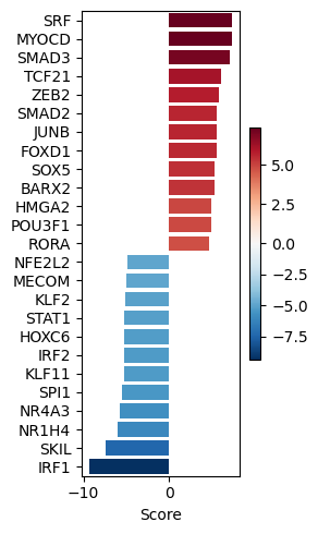
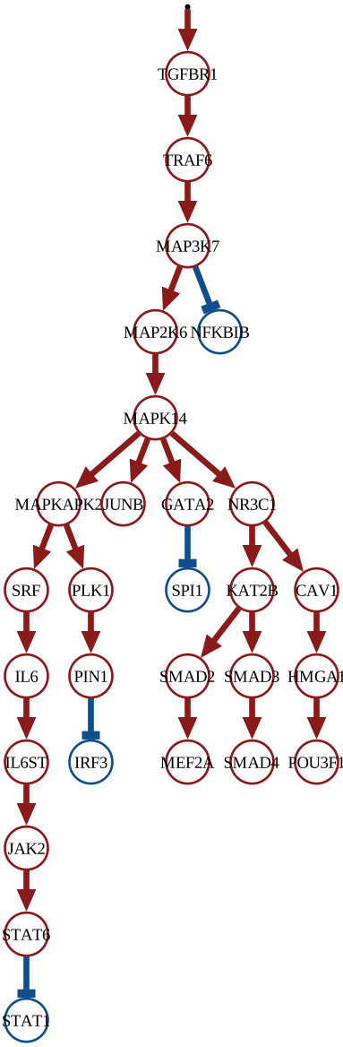
We will show how to estimate Transcription Factor activities from gene expression data, following the Decoupler tutorial for functional analysis. Then, we will use RIDDEN to estimate, in a similar fashion, receptor activities. Finally, we will use the CARNIVAL method available in CORNETO to infer a network from receptors to TFs, assuming that we don’t really know which treatment was used.
Please keep in mind that CARNIVAL, as any other method, is designed to facilitate systematic exploration of intracellular signalling hypotheses by leveraging curated knowledge-base networks. It is not intended to produce a single, definitive solution.
Parameter Sensitivity
Alterations in solver settings, threshold values, or choice of prior-knowledge networks can materially affect the inferred network.Data Dependence
The characteristics of your dataset—experimental design, sample size, preprocessing, and normalization—will directly influence model outputs.Knowledge-Base Limitations
Underlying pathway repositories may exhibit incomplete coverage and annotation biases.
Each network generated by CARNIVAL should be regarded as a potential, simplified hypothesis of the real signalling. Users are encouraged to compare multiple configurations and to validate the most promising models through further analysis and experimental validation.
NOTE: This tutorial uses the new Decoupler v2 version. We also use the highs free, open source solver, which has to be installed with
pip install highspy
import gzip
import os
import shutil
import tempfile
import urllib.request
import pandas as pd

# https://decoupler-py.readthedocs.io
import decoupler as dc
import numpy as np

# https://omnipathdb.org/
import omnipath as op

# Pydeseq for differential expression analysis
from pydeseq2.dds import DefaultInference, DeseqDataSet
from pydeseq2.ds import DeseqStats

# https://corneto.org
import corneto as cn
dc.__version__
'2.0.6'
max_time = 300
seed = 0
# Load the dataset
adata = dc.ds.hsctgfb()
adata
AnnData object with n_obs × n_vars = 6 × 58674
    obs: 'condition', 'sample_id'
Data preprocessing#
We will use AnnData and PyDeseq2 to pre-process the data and compute differential expression between control and tretament
# Obtain genes that pass the thresholds
dc.pp.filter_by_expr(
    adata=adata,
    group="condition",
    min_count=10,
    min_total_count=15,
    large_n=10,
    min_prop=0.7,
)
adata
AnnData object with n_obs × n_vars = 6 × 19510
    obs: 'condition', 'sample_id'
# Build DESeq2 object
inference = DefaultInference(n_cpus=8)
dds = DeseqDataSet(
    adata=adata,
    design_factors="condition",
    refit_cooks=True,
    inference=inference,
)

# Compute LFCs
dds.deseq2()

# Extract contrast between conditions
stat_res = DeseqStats(dds, contrast=["condition", "treatment", "control"], inference=inference)

# Compute Wald test
stat_res.summary()
Using None as control genes, passed at DeseqDataSet initialization
Log2 fold change & Wald test p-value: condition treatment vs control
                  baseMean  log2FoldChange     lfcSE       stat  \
RP11-347I19.8    88.877997       -0.207125  0.252557  -0.820110
TMEM170B        103.807801       -0.276960  0.210575  -1.315260
RP11-91P24.6    185.514929       -0.305848  0.180937  -1.690352
SLC33A1        2559.269047        0.595912  0.085253   6.989890
SNORA61          66.168502        0.746770  0.266470   2.802454
...                    ...             ...       ...        ...
RP11-75I2.3     771.828248        3.812419  0.128113  29.758231
SLC25A24       3525.523888        0.651017  0.087599   7.431750
BTN2A2          674.018191       -0.107905  0.106223  -1.015833
RP11-101E3.5    194.084339        0.092515  0.181973   0.508402
RP11-91I8.3      10.761886       -3.804532  0.920191  -4.134502

                      pvalue           padj
RP11-347I19.8   4.121536e-01   5.540987e-01
TMEM170B        1.884227e-01   3.053908e-01
RP11-91P24.6    9.096068e-02   1.682470e-01
SLC33A1         2.751015e-12   2.426415e-11
SNORA61         5.071542e-03   1.382697e-02
...                      ...            ...
RP11-75I2.3    1.357073e-194  4.412748e-192
SLC25A24        1.071704e-13   1.050701e-12
BTN2A2          3.097088e-01   4.492492e-01
RP11-101E3.5    6.111714e-01   7.290708e-01
RP11-91I8.3     3.557244e-05   1.474439e-04

[19510 rows x 6 columns]
results_df = stat_res.results_df
results_df
| baseMean | log2FoldChange | lfcSE | stat | pvalue | padj | |
|---|---|---|---|---|---|---|
| RP11-347I19.8 | 88.877997 | -0.207125 | 0.252557 | -0.820110 | 4.121536e-01 | 5.540987e-01 |
| TMEM170B | 103.807801 | -0.276960 | 0.210575 | -1.315260 | 1.884227e-01 | 3.053908e-01 |
| RP11-91P24.6 | 185.514929 | -0.305848 | 0.180937 | -1.690352 | 9.096068e-02 | 1.682470e-01 |
| SLC33A1 | 2559.269047 | 0.595912 | 0.085253 | 6.989890 | 2.751015e-12 | 2.426415e-11 |
| SNORA61 | 66.168502 | 0.746770 | 0.266470 | 2.802454 | 5.071542e-03 | 1.382697e-02 |
| ... | ... | ... | ... | ... | ... | ... |
| RP11-75I2.3 | 771.828248 | 3.812419 | 0.128113 | 29.758231 | 1.357073e-194 | 4.412748e-192 |
| SLC25A24 | 3525.523888 | 0.651017 | 0.087599 | 7.431750 | 1.071704e-13 | 1.050701e-12 |
| BTN2A2 | 674.018191 | -0.107905 | 0.106223 | -1.015833 | 3.097088e-01 | 4.492492e-01 |
| RP11-101E3.5 | 194.084339 | 0.092515 | 0.181973 | 0.508402 | 6.111714e-01 | 7.290708e-01 |
| RP11-91I8.3 | 10.761886 | -3.804532 | 0.920191 | -4.134502 | 3.557244e-05 | 1.474439e-04 |
19510 rows × 6 columns
data = results_df[["stat"]].T.rename(index={"stat": "treatment.vs.control"})
data
| RP11-347I19.8 | TMEM170B | RP11-91P24.6 | SLC33A1 | SNORA61 | THAP9-AS1 | LIX1L | TTC8 | WBSCR22 | LPHN2 | ... | STARD4-AS1 | ZNF845 | NIPSNAP3B | ARL6IP5 | MATN1-AS1 | RP11-75I2.3 | SLC25A24 | BTN2A2 | RP11-101E3.5 | RP11-91I8.3 | |
|---|---|---|---|---|---|---|---|---|---|---|---|---|---|---|---|---|---|---|---|---|---|
| treatment.vs.control | -0.82011 | -1.31526 | -1.690352 | 6.98989 | 2.802454 | 1.531175 | 2.164055 | -0.579835 | -0.945628 | -14.351065 | ... | 14.484178 | 0.567176 | -1.882852 | -8.425175 | -1.739571 | 29.758231 | 7.43175 | -1.015833 | 0.508402 | -4.134502 |
1 rows × 19510 columns
Estimation of Transcription Factor activities with Deocupler and CollecTRI#
# Retrieve CollecTRI gene regulatory network (through Omnipath).
# These are regulons that we will use for enrichment tests
# to infer TF activities
collectri = dc.op.collectri(organism="human")
collectri
| source | target | weight | resources | references | sign_decision | |
|---|---|---|---|---|---|---|
| 0 | MYC | TERT | 1.0 | DoRothEA-A;ExTRI;HTRI;NTNU.Curated;Pavlidis202... | 10022128;10491298;10606235;10637317;10723141;1... | PMID |
| 1 | SPI1 | BGLAP | 1.0 | ExTRI | 10022617 | default activation |
| 2 | SMAD3 | JUN | 1.0 | ExTRI;NTNU.Curated;TFactS;TRRUST | 10022869;12374795 | PMID |
| 3 | SMAD4 | JUN | 1.0 | ExTRI;NTNU.Curated;TFactS;TRRUST | 10022869;12374795 | PMID |
| 4 | STAT5A | IL2 | 1.0 | ExTRI | 10022878;11435608;17182565;17911616;22854263;2... | default activation |
| ... | ... | ... | ... | ... | ... | ... |
| 42985 | NFKB | hsa-miR-143-3p | 1.0 | ExTRI | 19472311 | default activation |
| 42986 | AP1 | hsa-miR-206 | 1.0 | ExTRI;GEREDB;NTNU.Curated | 19721712 | PMID |
| 42987 | NFKB | hsa-miR-21 | 1.0 | ExTRI | 20813833;22387281 | default activation |
| 42988 | NFKB | hsa-miR-224-5p | 1.0 | ExTRI | 23474441;23988648 | default activation |
| 42989 | AP1 | hsa-miR-144-3p | 1.0 | ExTRI | 23546882 | default activation |
42990 rows × 6 columns
# Run
tf_acts, tf_padj = dc.mt.ulm(data=data, net=collectri)

# Filter by sign padj
msk = (tf_padj.T < 0.05).iloc[:, 0]
tf_acts = tf_acts.loc[:, msk]

tf_acts
| APEX1 | ARID1A | ARID4B | ARNT | ASXL1 | ATF6 | BARX2 | BCL11A | BCL11B | BMAL2 | ... | TBX10 | TCF21 | TFAP2C | TP53 | VEZF1 | WWTR1 | ZBTB33 | ZEB2 | ZNF804A | ZXDC | |
|---|---|---|---|---|---|---|---|---|---|---|---|---|---|---|---|---|---|---|---|---|---|
| treatment.vs.control | -2.658269 | -3.915338 | -2.806407 | 3.170952 | 3.744263 | 2.705119 | 5.354716 | 2.647705 | -4.201891 | 3.866736 | ... | -3.703038 | 6.159527 | -2.57872 | -3.618243 | 4.205744 | -3.965664 | 3.235743 | 5.787311 | 3.363825 | -2.733078 |
1 rows × 142 columns
dc.pl.barplot(data=tf_acts, name="treatment.vs.control", top=25, figsize=(3, 5))
Estimation of Receptor activities with RIDDEN#
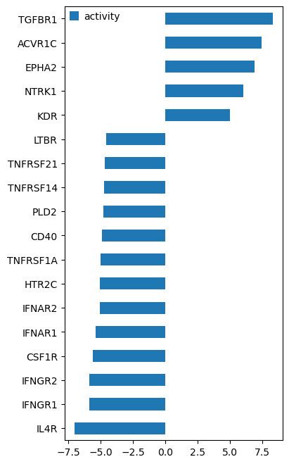
Now, we will use RIDDEN to estimate receptor activities. Here we know that the cells were treated with TGF-β, but we can assume that in general, this information might not be known. Let’s use RIDDEN with Decoupler to find out, from gene expression alone, which receptors seem to be responsible of the downstream changes in gene expression.
Barsi, S., Varga, E., Dimitrov, D., Saez-Rodriguez, J., Hunyady, L., & Szalai, B. (2025). RIDDEN: Data-driven inference of receptor activity from transcriptomic data. PLOS Computational Biology, 21(6), e1013188. https://journals.plos.org/ploscompbiol/article?id=10.1371/journal.pcbi.1013188
# We obtain ligand-receptor interactions from Omnipath, and we keep only the receptors
# This is our list of a prior potential receptors from which we will infer the network
unique_receptors = set(op.interactions.LigRecExtra.get(genesymbols=True)["target_genesymbol"].values.tolist())
len(unique_receptors)
1201
# We load the RIDDEN matrix
df_ridden = pd.read_csv(
    "https://github.com/basvaat/RIDDEN_tool/raw/aa3c9d9880f135e95a079865ee20ebec984cf54d/ridden_model/ridden_model_matrix.csv",
    index_col=0,
)
df_ridden
| GNPDA1 | CDH3 | HDAC6 | PARP2 | MAMLD1 | DNAJB6 | SMC4 | ABCC5 | ABCB6 | DNM1L | ... | NCAPD2 | PAN2 | LPGAT1 | KIF14 | CDC25A | CDC25B | OXSR1 | MVP | CDC42 | DMTF1 | |
|---|---|---|---|---|---|---|---|---|---|---|---|---|---|---|---|---|---|---|---|---|---|
| CALCRL | -0.009687 | -0.007085 | 0.161641 | -0.088799 | 0.141184 | 0.206650 | -0.077551 | 0.089438 | 0.052901 | -0.097550 | ... | -0.029438 | 0.093616 | -0.111194 | 0.055189 | -0.267147 | -0.132507 | 0.075775 | 0.206272 | -0.086620 | 0.089023 |
| IGF1R | 0.186149 | -0.019531 | -0.226755 | 0.241395 | -0.006143 | -0.195346 | -0.074546 | -0.110967 | -0.093491 | 0.144233 | ... | -0.092025 | -0.249430 | -0.090110 | -0.148717 | 0.507459 | -0.383608 | 0.080747 | -0.325099 | 0.122792 | -0.085241 |
| TEK | -0.184470 | 0.103735 | -0.178644 | 0.217038 | -0.030282 | -0.098075 | 0.457752 | 0.060260 | 0.101412 | 0.249132 | ... | -0.022321 | -0.144688 | -0.008170 | 0.418425 | 0.345027 | 0.257878 | 0.283288 | -0.180285 | 0.361584 | 0.121627 |
| GCGR | 0.154128 | -0.062489 | 0.193690 | 0.018437 | 0.037480 | 0.053541 | 0.120568 | 0.101133 | 0.055264 | -0.231345 | ... | -0.074465 | 0.546507 | -0.077048 | 0.118103 | 0.106227 | -0.102328 | -0.023940 | -0.072013 | 0.026697 | 0.201512 |
| AXL | -0.575718 | 0.078760 | -0.014661 | 0.292999 | 0.070583 | -0.012008 | 0.039746 | 0.006026 | 0.060853 | 0.119499 | ... | 0.236579 | -0.145577 | -0.109871 | 0.046791 | 0.301887 | -0.046162 | -0.022249 | -0.197795 | 0.319452 | 0.002319 |
| ... | ... | ... | ... | ... | ... | ... | ... | ... | ... | ... | ... | ... | ... | ... | ... | ... | ... | ... | ... | ... | ... |
| LAT | -0.090900 | -0.085613 | -0.050680 | 0.071466 | -0.020198 | -0.005307 | 0.152670 | 0.605020 | 0.339265 | -0.044672 | ... | 0.077842 | 0.541145 | -0.112621 | 0.378760 | -0.020636 | -0.188372 | -0.031565 | -0.447521 | 0.152605 | 0.233283 |
| KIR3DL2 | -0.113160 | -0.078494 | 0.076545 | -0.078937 | 0.243577 | -0.189946 | 0.286184 | 0.039433 | -0.174081 | -0.109293 | ... | -0.148066 | 0.118362 | 0.199176 | 0.109609 | 0.091345 | 0.243448 | 0.109597 | 0.032553 | 0.254494 | 0.058646 |
| ROR1 | -0.090646 | 0.012197 | -0.271497 | -0.158861 | 0.256878 | -0.078914 | -0.364736 | -0.012256 | -0.192445 | -0.670970 | ... | -0.005142 | -0.096561 | -0.262883 | -0.399374 | -0.109447 | -0.239205 | -0.257403 | 0.030898 | 0.098747 | 0.123366 |
| AGER | 0.020215 | 0.288864 | 0.214776 | -0.022412 | -0.038031 | -0.152819 | 0.157402 | 0.367379 | -0.038862 | -0.294257 | ... | -0.198762 | 0.227099 | 0.167598 | 0.154016 | 0.059484 | 0.124841 | 0.020183 | 0.083234 | 0.290658 | 0.194672 |
| LPAR4 | -0.207898 | -0.260550 | 0.091162 | 0.236077 | 0.242604 | -0.122191 | 0.661206 | -0.262016 | 0.296903 | -0.370393 | ... | -0.144404 | -0.132523 | 1.057903 | 0.216050 | 0.265133 | 0.621863 | 0.151718 | -0.158971 | 0.196567 | -0.274069 |
229 rows × 978 columns
df_receptor_de = data.loc[:, data.columns.intersection(df_ridden.columns)]
df_receptor_de
| CDC25B | CCNB2 | ABCC5 | NPDC1 | AGL | GMNN | BLCAP | ISOC1 | SLC35B1 | PAK1 | ... | HMGCR | LAMA3 | FAM57A | SSBP2 | CXCL2 | GTPBP8 | TRIB3 | HDAC2 | LGALS8 | BIRC5 | |
|---|---|---|---|---|---|---|---|---|---|---|---|---|---|---|---|---|---|---|---|---|---|
| treatment.vs.control | -8.391308 | 6.554248 | -4.139615 | -2.506713 | 0.299272 | 6.582295 | -2.918605 | -9.658493 | 3.163861 | 3.969934 | ... | 7.125527 | -3.862645 | 7.445228 | -8.977077 | -6.753168 | -5.144084 | 2.988088 | 5.638864 | -1.495224 | 6.237914 |
1 rows × 923 columns
ridden_pkn = df_ridden.reset_index().melt(id_vars="index")
ridden_pkn.columns = ["source", "target", "weight"]
ridden_pkn
| source | target | weight | |
|---|---|---|---|
| 0 | CALCRL | GNPDA1 | -0.009687 |
| 1 | IGF1R | GNPDA1 | 0.186149 |
| 2 | TEK | GNPDA1 | -0.184470 |
| 3 | GCGR | GNPDA1 | 0.154128 |
| 4 | AXL | GNPDA1 | -0.575718 |
| ... | ... | ... | ... |
| 223957 | LAT | DMTF1 | 0.233283 |
| 223958 | KIR3DL2 | DMTF1 | 0.058646 |
| 223959 | ROR1 | DMTF1 | 0.123366 |
| 223960 | AGER | DMTF1 | 0.194672 |
| 223961 | LPAR4 | DMTF1 | -0.274069 |
223962 rows × 3 columns
# Number of receptors in RIDDEN
len(ridden_pkn.source.unique())
229
# Run receptor enrichment with ULM
pw_acts, pw_padj = dc.mt.ulm(data=df_receptor_de, net=ridden_pkn)

df_ridden_stats = pd.concat([pw_acts, pw_padj]).T
df_ridden_stats.columns = ["activity", "padj"]
df_ridden_stats
| activity | padj | |
|---|---|---|
| ABCA1 | -3.208177 | 0.005754 |
| ACKR3 | 0.011038 | 0.992936 |
| ACTR2 | -0.732264 | 0.600567 |
| ACVR1 | 1.325987 | 0.321247 |
| ACVR1B | 3.472131 | 0.002690 |
| ... | ... | ... |
| TRAF2 | -3.728965 | 0.001258 |
| TYRO3 | -2.533851 | 0.033606 |
| UTS2R | -4.147080 | 0.000334 |
| VIPR1 | 1.316101 | 0.324505 |
| XCR1 | -1.251474 | 0.338022 |
229 rows × 2 columns
# We inferred from gene expression that TGFBR1 is the most active receptor
df_ridden_stats[df_ridden_stats.padj <= 0.0001][["activity"]].sort_values(by="activity", ascending=True).plot.barh(
    figsize=(4, 8)
)
<Axes: >
Inferring intracellular signalling network with CARNIVAL and CORNETO#
CORNETO is a unified framework for knowledge-driven network inference. It includes a very flexible implementation of CARNIVAL that expands its original capabilities. We will see how to use it under different assumptions to extract a network from a prior knowledge network and a set of potential receptors + our estimated TFs
cn.info()

|
|
from corneto.methods import CarnivalFlow

CarnivalFlow.show_references()
- Pablo Rodriguez-Mier, Martin Garrido-Rodriguez, Attila Gabor, Julio Saez-Rodriguez. Unified knowledge-driven network inference from omics data. bioRxiv, pp. 10 (2024).
- Anika Liu, Panuwat Trairatphisan, Enio Gjerga, Athanasios Didangelos, Jonathan Barratt, Julio Saez-Rodriguez. From expression footprints to causal pathways: contextualizing large signaling networks with CARNIVAL. NPJ systems biology and applications, Vol. 5, No. 1, pp. 40 (2019).
# We get only interactions from SIGNOR http://signor.uniroma2.it/
pkn = op.interactions.OmniPath.get(databases=["SIGNOR"], genesymbols=True)
pkn = pkn[pkn.consensus_direction == True]
pkn.head()
| source | target | source_genesymbol | target_genesymbol | is_directed | is_stimulation | is_inhibition | consensus_direction | consensus_stimulation | consensus_inhibition | curation_effort | references | sources | n_sources | n_primary_sources | n_references | references_stripped | |
|---|---|---|---|---|---|---|---|---|---|---|---|---|---|---|---|---|---|
| 0 | Q13976 | Q13507 | PRKG1 | TRPC3 | True | False | True | True | False | True | 9 | HPRD:14983059;KEA:14983059;ProtMapper:14983059... | HPRD;HPRD_KEA;HPRD_MIMP;KEA;MIMP;PhosphoPoint;... | 15 | 8 | 2 | 14983059;16331690 |
| 1 | Q13976 | Q9HCX4 | PRKG1 | TRPC7 | True | True | False | True | True | False | 3 | SIGNOR:21402151;TRIP:21402151;iPTMnet:21402151 | SIGNOR;TRIP;iPTMnet | 3 | 3 | 1 | 21402151 |
| 2 | Q13438 | Q9HBA0 | OS9 | TRPV4 | True | True | True | True | True | True | 3 | HPRD:17932042;SIGNOR:17932042;TRIP:17932042 | HPRD;SIGNOR;TRIP | 3 | 3 | 1 | 17932042 |
| 3 | P18031 | Q9H1D0 | PTPN1 | TRPV6 | True | False | True | True | False | True | 11 | DEPOD:15894168;DEPOD:17197020;HPRD:15894168;In... | DEPOD;HPRD;IntAct;Lit-BM-17;SIGNOR;SPIKE_LC;TRIP | 7 | 6 | 2 | 15894168;17197020 |
| 4 | P63244 | Q9BX84 | RACK1 | TRPM6 | True | False | True | True | False | True | 2 | SIGNOR:18258429;TRIP:18258429 | SIGNOR;TRIP | 2 | 2 | 1 | 18258429 |
pkn["interaction"] = pkn["is_stimulation"].astype(int) - pkn["is_inhibition"].astype(int)
sel_pkn = pkn[["source_genesymbol", "interaction", "target_genesymbol"]]
sel_pkn
| source_genesymbol | interaction | target_genesymbol | |
|---|---|---|---|
| 0 | PRKG1 | -1 | TRPC3 |
| 1 | PRKG1 | 1 | TRPC7 |
| 2 | OS9 | 0 | TRPV4 |
| 3 | PTPN1 | -1 | TRPV6 |
| 4 | RACK1 | -1 | TRPM6 |
| ... | ... | ... | ... |
| 61542 | APC_PUF60_SIAH1_SKP1_TBL1X | -1 | CTNNB1 |
| 61543 | MAP2K6 | 1 | MAPK10 |
| 61544 | PRKAA1 | 1 | TP53 |
| 61545 | CNOT1_CNOT10_CNOT11_CNOT2_CNOT3_CNOT4_CNOT6_CN... | -1 | NANOS2 |
| 61546 | WNT16 | 1 | FZD3 |
60921 rows × 3 columns
# We create the CORNETO graph by importing the edges and interaction
from corneto.io import load_graph_from_sif_tuples

G = load_graph_from_sif_tuples([(r[0], r[1], r[2]) for _, r in sel_pkn.iterrows() if r[1] != 0])
G.shape
(5442, 60034)
# As measurements, we take the estimated TFs, we will filter out TFs with p-val > 0.001
significant_tfs = tf_acts[tf_padj <= 0.001].T.dropna().sort_values(by="treatment.vs.control", ascending=False)
significant_tfs
| treatment.vs.control | |
|---|---|
| SRF | 7.390611 |
| MYOCD | 7.342673 |
| SMAD3 | 7.084429 |
| TCF21 | 6.159527 |
| ZEB2 | 5.787311 |
| SMAD2 | 5.614428 |
| JUNB | 5.610473 |
| FOXD1 | 5.566138 |
| SOX5 | 5.385469 |
| BARX2 | 5.354716 |
| HMGA2 | 4.918146 |
| POU3F1 | 4.903790 |
| RORA | 4.748799 |
| SMAD4 | 4.440260 |
| OVOL1 | 4.280655 |
| MEF2A | 4.232877 |
| FGF2 | 4.207762 |
| VEZF1 | 4.205744 |
| EGR4 | 4.110464 |
| SMAD5 | -4.004015 |
| CIITA | -4.133309 |
| NFKBIB | -4.154074 |
| REL | -4.165033 |
| PITX3 | -4.198049 |
| BCL11B | -4.201891 |
| IRF3 | -4.272800 |
| PITX1 | -4.340665 |
| PARK7 | -4.445422 |
| KLF8 | -4.467109 |
| DNMT3A | -4.622450 |
| RELB | -4.681916 |
| NFE2L2 | -4.911003 |
| MECOM | -4.942362 |
| KLF2 | -5.094150 |
| STAT1 | -5.189259 |
| HOXC6 | -5.215468 |
| IRF2 | -5.269444 |
| KLF11 | -5.269653 |
| SPI1 | -5.431022 |
| NR4A3 | -5.723505 |
| NR1H4 | -6.055603 |
| SKIL | -7.433282 |
| IRF1 | -9.357501 |
# We keep only the ones in the PKN graph
measurements = significant_tfs.loc[significant_tfs.index.intersection(G.V)].to_dict()["treatment.vs.control"]
measurements
{'SRF': 7.3906108743123164,
 'MYOCD': 7.342672817892572,
 'SMAD3': 7.0844294103820795,
 'ZEB2': 5.787311392244455,
 'SMAD2': 5.614427728369875,
 'JUNB': 5.610473028026834,
 'HMGA2': 4.918146140281221,
 'POU3F1': 4.903790337294035,
 'RORA': 4.748799034758163,
 'SMAD4': 4.4402600755156145,
 'MEF2A': 4.232877334898612,
 'FGF2': 4.207761616198675,
 'SMAD5': -4.004015430616565,
 'CIITA': -4.133309143328191,
 'NFKBIB': -4.154074213081593,
 'REL': -4.165033347663166,
 'PITX3': -4.198048894427097,
 'IRF3': -4.272799795168503,
 'PITX1': -4.340665200624415,
 'KLF8': -4.467109049496403,
 'DNMT3A': -4.622449958822471,
 'RELB': -4.681915557899264,
 'NFE2L2': -4.911003015915443,
 'MECOM': -4.942361740804518,
 'STAT1': -5.189258911506045,
 'HOXC6': -5.2154678064628905,
 'IRF2': -5.269444375678524,
 'KLF11': -5.269652535831714,
 'SPI1': -5.431022120705177,
 'NR4A3': -5.72350500604796,
 'NR1H4': -6.055602968386476,
 'SKIL': -7.433281684514384,
 'IRF1': -9.357500631318382}
"TGFBR1" in G.V
True
# Here we pass the receptors. We're going to use the top receptor inferred by RIDDEN
# (TGFBR1)
inputs = {"TGFBR1": 1}  # 1=up, -1=down
inputs
{'TGFBR1': 1}
# Create the dataset in standard format
carnival_data = dict()
for inp, v in inputs.items():
    carnival_data[inp] = dict(value=v, role="input", mapping="vertex")
for out, v in measurements.items():
    carnival_data[out] = dict(value=v, role="output", mapping="vertex")
data = cn.Data.from_cdict({"sample1": carnival_data})
data
Data(n_samples=1, n_feats=[34])
CARNIVAL#
We will use now the CARNIVAL, as implemented with CORNETO, with a penalty to regularize the solution. For hypothesis exploration, we can try different values and manually inspect the solutions. We are going to penalize also the selection of indirect rules, to simplify the solution. These rules are:
A -> B in the PKN, and we observe B is downregulated, we explain it with downregulation of its upstream gene A
A -| B in the PKN, and we observe B is upregulated, we explain it with downregulation of A
carnival = CarnivalFlow(lambda_reg=1.0, indirect_rule_penalty=10)
P = carnival.build(G, data)
P.expr
Unreachable vertices for sample: 0
{'_flow': _flow: Variable((3251,), _flow),
 'edge_activates': edge_activates: Variable((3251, 1), edge_activates, boolean=True),
 'edge_inhibits': edge_inhibits: Variable((3251, 1), edge_inhibits, boolean=True),
 'const0x689caa490bb1d38': const0x689caa490bb1d38: Constant(CONSTANT, NONNEGATIVE, (937, 3251)),
 '_dag_layer': _dag_layer: Variable((937, 1), _dag_layer),
 'const0x1f364c592f0a234': const0x1f364c592f0a234: Constant(CONSTANT, NONNEGATIVE, (937, 3251)),
 'flow': _flow: Variable((3251,), _flow),
 'vertex_value': Expression(AFFINE, UNKNOWN, (937, 1)),
 'vertex_activated': Expression(AFFINE, NONNEGATIVE, (937, 1)),
 'vertex_inhibited': Expression(AFFINE, NONNEGATIVE, (937, 1)),
 'edge_value': Expression(AFFINE, UNKNOWN, (3251, 1)),
 'edge_has_signal': Expression(AFFINE, NONNEGATIVE, (3251, 1)),
 'vertex_max_depth': _dag_layer: Variable((937, 1), _dag_layer)}
P.solve(solver="highs", max_seconds=60, verbosity=1);
===============================================================================
                                     CVXPY
                                     v1.7.1
===============================================================================
-------------------------------------------------------------------------------
                                  Compilation
-------------------------------------------------------------------------------
-------------------------------------------------------------------------------
                                Numerical solver
-------------------------------------------------------------------------------
Running HiGHS 1.11.0 (git hash: 364c83a): Copyright (c) 2025 HiGHS under MIT licence terms
MIP  has 30607 rows; 10690 cols; 108040 nonzeros; 6502 integer variables (6502 binary)
Coefficient ranges:
  Matrix [1e+00, 9e+02]
  Cost   [1e+00, 2e+01]
  Bound  [1e+00, 1e+00]
  RHS    [1e+00, 1e+03]
Presolving model
17785 rows, 10295 cols, 91250 nonzeros  0s
12839 rows, 9091 cols, 69193 nonzeros  0s
12451 rows, 9010 cols, 68715 nonzeros  0s

Solving MIP model with:
   12451 rows
   9010 cols (5622 binary, 0 integer, 0 implied int., 3388 continuous, 0 domain fixed)
   68715 nonzeros

Src: B => Branching; C => Central rounding; F => Feasibility pump; J => Feasibility jump;
     H => Heuristic; L => Sub-MIP; P => Empty MIP; R => Randomized rounding; Z => ZI Round;
     I => Shifting; S => Solve LP; T => Evaluate node; U => Unbounded; X => User solution;
     z => Trivial zero; l => Trivial lower; u => Trivial upper; p => Trivial point

        Nodes      |    B&B Tree     |            Objective Bounds              |  Dynamic Constraints |       Work
Src  Proc. InQueue |  Leaves   Expl. | BestBound       BestSol              Gap |   Cuts   InLp Confl. | LpIters     Time

         0       0         0   0.00%   -65.07953075    inf                  inf        0      0      0         0     0.5s
         0       0         0   0.00%   -35.74261013    inf                  inf        0      0      0       916     0.6s
 C       0       0         0   0.00%   -31.4613484     1               3246.13%      174     21      0      1033     1.2s
 L       0       0         0   0.00%   -31.4613484     -27.4613484       14.57%      337     28      0      1074     3.4s

59.7% inactive integer columns, restarting
Model after restart has 4812 rows, 4314 cols (1316 bin., 0 int., 0 impl., 2998 cont., 0 dom.fix.), and 20181 nonzeros

         0       0         0   0.00%   -31.4613484     -27.4613484       14.57%       12      0      0      6233     4.1s
         0       0         0   0.00%   -31.4613484     -27.4613484       14.57%       12     10      0      6344     4.1s
 L       0       0         0   0.00%   -31.4613484     -29.4613484        6.79%      282     28      0      6442     5.0s

2.5% inactive integer columns, restarting
Model after restart has 4517 rows, 4177 cols (1220 bin., 0 int., 0 impl., 2957 cont., 0 dom.fix.), and 19933 nonzeros

         0       0         0   0.00%   -31.4613484     -29.4613484        6.79%       15      0      0     14641     5.3s
         0       0         0   0.00%   -31.4613484     -29.4613484        6.79%       15      3      3     14727     5.3s

6.6% inactive integer columns, restarting
Model after restart has 4106 rows, 3960 cols (1096 bin., 0 int., 0 impl., 2864 cont., 0 dom.fix.), and 17942 nonzeros

         0       0         0   0.00%   -30.89268612    -29.4613484        4.86%       16      0      0     14945     5.4s
         0       0         0   0.00%   -30.89268612    -29.4613484        4.86%       16     12     10     15011     5.4s

Symmetry detection completed in 0.0s
Found 7 generator(s)

Restarting search from the root node
Model after restart has 1218 rows, 2727 cols (172 bin., 0 int., 0 impl., 2555 cont., 0 dom.fix.), and 7817 nonzeros

        20       0         0   0.00%   -30.4613484     -29.4613484        3.39%       17      0      0     18065     6.0s
 R      20       0         0   0.00%   -30.4613484     -30.32402383       0.45%       17      6      0     18569     6.0s

33.7% inactive integer columns, restarting
Model after restart has 999 rows, 2632 cols (105 bin., 0 int., 0 impl., 2527 cont., 0 dom.fix.), and 7136 nonzeros

        20       0         0   0.00%   -30.4613484     -30.32402383       0.45%        6      0      0     18569     6.0s
        20       0         0   0.00%   -30.4613484     -30.32402383       0.45%        6      4      3     18955     6.0s

10.5% inactive integer columns, restarting
Model after restart has 950 rows, 2611 cols (92 bin., 0 int., 0 impl., 2519 cont., 0 dom.fix.), and 6975 nonzeros

        20       0         0   0.00%   -30.4613484     -30.32402383       0.45%        5      0      0     18957     6.0s
        20       0         0   0.00%   -30.4613484     -30.32402383       0.45%        5      5      8     19024     6.0s

Symmetry detection completed in 0.0s
No symmetry present

        31       0         6 100.00%   -30.32402383    -30.32402383       0.00%      402     16     23     19451     6.1s

Solving report
  Status            Optimal
  Primal bound      -30.3240238293
  Dual bound        -30.3240238293
  Gap               0% (tolerance: 0.01%)
  P-D integral      73.2418044379
  Solution status   feasible
                    -30.3240238293 (objective)
                    0 (bound viol.)
                    0 (int. viol.)
                    0 (row viol.)
  Timing            6.10 (total)
                    0.00 (presolve)
                    0.00 (solve)
                    0.00 (postsolve)
  Max sub-MIP depth 7
  Nodes             31
  Repair LPs        0 (0 feasible; 0 iterations)
  LP iterations     19451 (total)
                    2003 (strong br.)
                    1132 (separation)
                    13344 (heuristics)
-------------------------------------------------------------------------------
                                    Summary
-------------------------------------------------------------------------------
# Error for sample is 0, meaning that all reachable TFs (from receptors) are correctly explained
for o in P.objectives:
    print(o.name, "->", o.value)
error_sample1_0 -> 64.98036838411093
penalty_indirect_rules_0 -> [0.]
regularization_edge_has_signal -> 28.0
# We extract the selected edges
sol_edges = np.flatnonzero(np.abs(P.expr.edge_value.value) > 0.5)
carnival.processed_graph.plot_values(
    vertex_values=P.expr.vertex_value.value,
    edge_values=P.expr.edge_value.value,
    edge_indexes=sol_edges,
)
# Extracting the solution graph
G_sol = carnival.processed_graph.edge_subgraph(sol_edges)
G_sol.shape
(28, 28)
pd.DataFrame(
    P.expr.vertex_value.value,
    index=carnival.processed_graph.V,
    columns=["node_activity"],
)
| node_activity | |
|---|---|
| P0DTC2_UBB | 0.0 |
| HRH1 | 0.0 |
| ATM | 0.0 |
| TNFRSF1A | 0.0 |
| RAC1 | 0.0 |
| ... | ... |
| PCBP2 | 0.0 |
| MAF | 0.0 |
| MAP3K1 | 0.0 |
| ARHGEF7 | 0.0 |
| GAB2 | 0.0 |
937 rows × 1 columns
pd.DataFrame(P.expr.edge_value.value, index=carnival.processed_graph.E, columns=["edge_activity"])
| edge_activity | ||
|---|---|---|
| (SMAD3) | (MYOD1) | 0.0 |
| (GRK2) | (BDKRB2) | 0.0 |
| (MAPK14) | (MAPKAPK2) | 1.0 |
| (DEPTOR_EEF1A1_MLST8_MTOR_PRR5_RICTOR) | (FBXW8) | 0.0 |
| (SLK) | (MAP3K5) | 0.0 |
| ... | ... | ... |
| (REL) | () | 0.0 |
| (MYOCD) | () | 0.0 |
| (RORA) | () | 0.0 |
| (IRF3) | () | 0.0 |
| () | (TGFBR1) | 1.0 |
3251 rows × 1 columns
Saving the processed dataset#
cn.GraphData(G, data).save("data/carnival_transcriptomics_dataset")