Multi-condition signalling network inference

In this notebook we show how to infer signalling networks for a multicondition setting.
Here we will use mouse RNA-seq data of a multicondition study, where we will compare normal to spontaneous leukemia and Sleeping-Beauty (SB) mediated leukemia.

In the first part, we will show how to estimate Transcription Factor activities from gene expression data, following the Decoupler tutorial for functional analysis.
Then, we will infer 2 networks for each of the 2 conditions and analyse differences.

• Author: Irene Rigato (Francesca Finotello’s group)

• Reviewers: Sophia Müller-Dott, Pablo Rodriguez-Mier

# --- Saezlab tools ---
# https://decoupler-py.readthedocs.io/
import gzip
import os
import shutil
import tempfile
import urllib.request

import decoupler as dc
import numpy as np

# https://omnipathdb.org/
import omnipath as op

# Additional packages
import pandas as pd

# --- Additional libs ---
# Pydeseq for differential expression analysis
from pydeseq2.dds import DefaultInference, DeseqDataSet
from pydeseq2.ds import DeseqStats

# https://saezlab.github.io/
import corneto as cn

cn.info()

Installed version: v1.0.0rc5 Available backends: CVXPY v1.9.1 Default backend (corneto.opt): CVXPY Installed solvers: CLARABEL, SCS, GUROBI, SCIPY, HIGHS, OSQP Plot backend (default): auto -> graphviz Available plot backends: graphviz v0.21; graphviz-wasm Installed path: /docs/tutorials/contrib/multi_condition_tutorial/.pixi/envs/default/lib/python3.11/site-packages/corneto Repository: https://github.com/saezlab/corneto

max_time = 300
seed = 0

# loading GEO GSE148679 dataset
url = "https://www.ncbi.nlm.nih.gov/geo/download/?acc=GSE148679&format=file&file=GSE148679%5Fcounts%5Fgsea%5Fanalysis%2Etxt%2Egz"

adata = None
with tempfile.TemporaryDirectory() as tmpdirname:
    # Path for the gzipped file in the temp folder
    gz_file_path = os.path.join(tmpdirname, "counts.txt.gz")

    # Download the file
    with urllib.request.urlopen(url) as response:
        with open(gz_file_path, "wb") as out_file:
            shutil.copyfileobj(response, out_file)

    # Decompress the file
    decompressed_file_path = gz_file_path[:-3]  # Removing '.gz' extension
    with gzip.open(gz_file_path, "rb") as f_in:
        with open(decompressed_file_path, "wb") as f_out:
            shutil.copyfileobj(f_in, f_out)

    adata = pd.read_csv(decompressed_file_path, index_col=0, sep="\t").T

adata.head()

ID	Itm2a	Sergef	Fam109a	Dhx9	Fam71e2	Ssu72	Olfr1018	Eif2b2	Mks1	Hebp2	...	Olfr372	Gosr1	Ctsw	Ryk	Rhd	Pxmp4	Gm25500	4930455C13Rik	Prss39	Reg4
Ebf1.1	265	332	306	27823	0	2969	0	2614	231	6	...	0	2967	674	150	708	830	29	9	7	0
Ebf1.2	175	471	335	35978	0	3108	0	2924	192	0	...	0	2724	155	142	869	867	5	4	16	0
Ebf1.3	266	382	325	30367	0	3207	0	2940	211	7	...	0	2547	87	54	291	767	7	7	6	0
Ebf1.4	212	388	331	30406	0	3168	0	2871	209	8	...	0	2568	169	115	1244	829	5	1	4	0
PE.1	321	312	290	22272	0	2631	0	2236	109	10	...	0	2466	837	191	921	888	2	2	8	0

5 rows × 24420 columns

from anndata import AnnData

adata = AnnData(adata, dtype=np.float32)
adata.var_names_make_unique()
adata

AnnData object with n_obs × n_vars = 53 × 24420

# Assign conditions explicitly. No sample is silently assigned to the control group.
sample_ids = adata.obs_names.to_series()
is_normal = sample_ids.str.match(r"^(WT|Pax5|Ebf1|PE\.\d+$)")
is_spontaneous = sample_ids.str.match(r"^PE\.Leuk\.")
is_sb = sample_ids.str.match(r"^SB")

membership_count = np.column_stack([is_normal, is_spontaneous, is_sb]).sum(axis=1)
if not np.all(membership_count == 1):
    invalid = sample_ids.index[membership_count != 1].tolist()
    raise ValueError(f"Samples with ambiguous or unknown condition: {invalid}")

adata.obs["condition"] = np.select(
    [is_normal, is_spontaneous, is_sb],
    ["Normal", "Leukemic_spontaneous", "Leukemic_SB"],
    default="Unknown",
)
adata.obs["condition"].value_counts()

condition
Leukemic_SB             31
Normal                  15
Leukemic_spontaneous     7
Name: count, dtype: int64

Splitting data for network inference and validation

Both contrasts use a fixed stratified holdout for lambda selection. The normal split is shared so condition scores remain comparable.

# Use a fixed, stratified biological holdout for lambda selection.
# The normal split is shared by both contrasts.
rng = np.random.default_rng(seed)


def train_validation_ids(ids, validation_fraction=0.25):
    ids = np.asarray(sorted(ids), dtype=object)
    ids = ids[rng.permutation(len(ids))]
    n_validation = max(2, int(round(len(ids) * validation_fraction)))
    n_validation = min(n_validation, len(ids) - 2)
    return ids[n_validation:], ids[:n_validation]


normal_ids = adata.obs_names[adata.obs["condition"] == "Normal"]
spontaneous_ids = adata.obs_names[adata.obs["condition"] == "Leukemic_spontaneous"]
sb_ids = adata.obs_names[adata.obs["condition"] == "Leukemic_SB"]

normal_train, normal_validation = train_validation_ids(normal_ids)
spontaneous_train, spontaneous_validation = train_validation_ids(spontaneous_ids)
sb_train, sb_validation = train_validation_ids(sb_ids)

adata1 = adata[list(normal_train) + list(spontaneous_train)].copy()
adata2 = adata[list(normal_train) + list(sb_train)].copy()
validation_adata1 = adata[list(normal_validation) + list(spontaneous_validation)].copy()
validation_adata2 = adata[list(normal_validation) + list(sb_validation)].copy()

pd.DataFrame(
    {
        "contrast": ["spontaneous", "SB"],
        "train_normal": [len(normal_train)] * 2,
        "train_disease": [len(spontaneous_train), len(sb_train)],
        "validation_normal": [len(normal_validation)] * 2,
        "validation_disease": [len(spontaneous_validation), len(sb_validation)],
    }
)

	contrast	train_normal	train_disease	validation_normal	validation_disease
0	spontaneous	11	5	4	2
1	SB	11	23	4	8

Differential expression analysis per condition

Contrast 1: Leukemic_spontaneous vs Normal

# Obtain genes that pass the thresholds
dc.pp.filter_by_expr(
    adata1,
    group="condition",
    min_count=10,
    min_total_count=15,
    large_n=10,
    min_prop=0.8,
)
adata1

AnnData object with n_obs × n_vars = 16 × 13599
    obs: 'condition'

# Estimation of differential expression
inference1 = DefaultInference()
dds1 = DeseqDataSet(
    adata=adata1,
    design_factors="condition",
    refit_cooks=True,
    inference=inference1,
)
dds1.deseq2()

Using None as control genes, passed at DeseqDataSet initialization

stat_res_leu1 = DeseqStats(dds1, contrast=["condition", "Leukemic_spontaneous", "Normal"], inference=inference1)

stat_res_leu1.summary()

Log2 fold change & Wald test p-value: condition Leukemic_spontaneous vs Normal
             baseMean  log2FoldChange     lfcSE       stat        pvalue  \
ID                                                                         
Itm2a      297.542647        0.893484  0.215371   4.148578  3.345473e-05   
Sergef     516.318790        1.271089  0.118853  10.694655  1.078196e-26   
Fam109a    340.369933        0.246593  0.111188   2.217812  2.656763e-02   
Dhx9     28163.396930       -0.038032  0.069192  -0.549658  5.825541e-01   
Ssu72     2932.274736        0.002847  0.056434   0.050457  9.597584e-01   
...               ...             ...       ...        ...           ...   
Ryk         77.201401       -2.781647  0.394009  -7.059862  1.666677e-12   
Rhd        378.982439       -4.297269  0.470384  -9.135671  6.500233e-20   
Pxmp4      787.520768       -0.381142  0.089869  -4.241074  2.224523e-05   
Gm25500      9.541753        0.665993  0.526790   1.264247  2.061412e-01   
Prss39       7.693766        0.742798  0.663470   1.119565  2.628993e-01   

                 padj  
ID                     
Itm2a    7.810706e-05  
Sergef   2.958178e-25  
Fam109a  3.984264e-02  
Dhx9     6.351182e-01  
Ssu72    9.670747e-01  
...               ...  
Ryk      9.404290e-12  
Rhd      8.472136e-19  
Pxmp4    5.345232e-05  
Gm25500  2.544401e-01  
Prss39   3.158001e-01  

[13599 rows x 6 columns]

results_df1 = stat_res_leu1.results_df
results_df1.sort_values(by="padj", ascending=True, inplace=False).head()

	baseMean	log2FoldChange	lfcSE	stat	pvalue	padj
ID
P2ry13	850.345057	3.279132	0.139851	23.447320	1.407802e-121	9.559678e-118
Zfp518b	587.950374	-7.670839	0.327080	-23.452452	1.247909e-121	9.559678e-118
Blvrb	1843.921725	-3.118163	0.139554	-22.343761	1.388454e-110	6.285531e-107
Kif19a	326.577342	-5.914527	0.269931	-21.911251	2.029295e-106	6.889963e-103
Zbtb42	319.477801	-2.080728	0.099745	-20.860557	1.222398e-96	3.320278e-93

Contrast 2: Leukemic_SB vs Normal

# Obtain genes that pass the thresholds
dc.pp.filter_by_expr(
    adata2,
    group="condition",
    min_count=10,
    min_total_count=15,
    large_n=10,
    min_prop=0.8,
)
adata2

AnnData object with n_obs × n_vars = 34 × 13286
    obs: 'condition'

# Estimation of differential expression
inference2 = DefaultInference()
dds2 = DeseqDataSet(
    adata=adata2,
    design_factors="condition",
    refit_cooks=True,
    inference=inference2,
)
dds2.deseq2()

Using None as control genes, passed at DeseqDataSet initialization

stat_res_leu2 = DeseqStats(dds2, contrast=["condition", "Leukemic_SB", "Normal"], inference=inference2)

stat_res_leu2.summary()

Log2 fold change & Wald test p-value: condition Leukemic_SB vs Normal
             baseMean  log2FoldChange     lfcSE       stat        pvalue  \
ID                                                                         
Itm2a      354.819498        0.814702  0.274887   2.963769  3.038960e-03   
Sergef     690.444712        1.247942  0.089243  13.983566  1.963960e-44   
Fam109a    372.293652        0.304612  0.105585   2.884977  3.914420e-03   
Dhx9     28125.836843       -0.017291  0.070394  -0.245630  8.059687e-01   
Ssu72     2943.414653        0.012841  0.071734   0.179011  8.579288e-01   
...               ...             ...       ...        ...           ...   
Ctsw       152.509072       -1.282962  0.455445  -2.816943  4.848307e-03   
Ryk         48.834169       -2.269091  0.335420  -6.764932  1.333718e-11   
Rhd        192.158985       -4.350260  0.483113  -9.004647  2.163614e-19   
Pxmp4      779.412902       -0.184564  0.117464  -1.571242  1.161264e-01   
Gm25500      8.770752        0.167093  0.366501   0.455914  6.484515e-01   

                 padj  
ID                     
Itm2a    5.951595e-03  
Sergef   2.438614e-42  
Fam109a  7.476564e-03  
Dhx9     8.450873e-01  
Ssu72    8.875218e-01  
...               ...  
Ctsw     9.094254e-03  
Ryk      8.976585e-11  
Rhd      3.401867e-18  
Pxmp4    1.596332e-01  
Gm25500  7.073339e-01  

[13286 rows x 6 columns]

results_df2 = stat_res_leu2.results_df
results_df2.sort_values(by="padj", ascending=True, inplace=False).head()

	baseMean	log2FoldChange	lfcSE	stat	pvalue	padj
ID
Mfsd2b	2514.371164	-9.636851	0.378623	-25.452370	6.645556e-143	8.829286e-139
Pf4	3805.666665	-13.199275	0.541930	-24.356055	5.001204e-131	3.322300e-127
Itga2b	9515.339854	-12.057495	0.503300	-23.956866	7.836582e-127	3.470561e-123
Ppbp	19266.371435	-16.866204	0.706022	-23.889076	3.978005e-126	1.321294e-122
Adgrl4	133.471953	-9.102316	0.387205	-23.507763	3.397368e-122	9.027486e-119

def fit_validation_de(adata_subset, disease_condition):
    validation = adata_subset.copy()
    dc.pp.filter_by_expr(
        validation,
        group="condition",
        min_count=10,
        min_total_count=15,
        large_n=10,
        min_prop=0.5,
    )
    inference = DefaultInference()
    dds = DeseqDataSet(
        adata=validation,
        design="~condition",
        refit_cooks=False,
        inference=inference,
        quiet=True,
    )
    dds.deseq2()
    stats = DeseqStats(
        dds,
        contrast=["condition", disease_condition, "Normal"],
        inference=inference,
        quiet=True,
    )
    stats.summary()
    return stats.results_df


validation_results_df1 = fit_validation_de(
    validation_adata1, "Leukemic_spontaneous"
)
validation_results_df2 = fit_validation_de(validation_adata2, "Leukemic_SB")

pd.DataFrame(
    {
        "condition": ["spontaneous", "SB"],
        "validation_genes": [len(validation_results_df1), len(validation_results_df2)],
    }
)

	condition	validation_genes
0	spontaneous	13739
1	SB	13536

Prior knowledge with Decoupler and Omnipath

# Retrieve native mouse CollecTRI interactions through OmniPath.
# This avoids a fragile human-to-mouse translation download.
collectri_raw = op.interactions.CollecTRI.get(organisms="mouse", genesymbols=True)
collectri = collectri_raw.assign(
    source=collectri_raw["source_genesymbol"],
    target=collectri_raw["target_genesymbol"],
    weight=(
        collectri_raw["consensus_stimulation"].astype(int)
        - collectri_raw["consensus_inhibition"].astype(int)
    ),
)[["source", "target", "weight"]]
collectri = collectri.loc[collectri["weight"] != 0].drop_duplicates()
collectri.head()

	source	target	weight
0	Myc	Tert	1
1	Spi1	Bglap2	1
2	Spi1	Bglap	1
3	Spi1	Bglap3	1
4	Smad3	Jun	1

TF activity inference per condition

Contrast 1: Leukemic_spontaneous vs Normal

mat1 = results_df1[["stat"]].T.rename(index={"stat": "Leukemic_spontaneous.vs.Normal"})
mat1

ID	Itm2a	Sergef	Fam109a	Dhx9	Ssu72	Eif2b2	Mks1	Vps28	Setd6	Gstm2	...	Rag2	Itgb1bp2	Sec23ip	Gosr1	Ctsw	Ryk	Rhd	Pxmp4	Gm25500	Prss39
Leukemic_spontaneous.vs.Normal	4.148578	10.694655	2.217812	-0.549658	0.050457	5.610092	5.178963	3.846342	8.079712	-2.671615	...	-4.541439	-0.473154	-9.441182	1.012695	-1.222221	-7.059862	-9.135671	-4.241074	1.264247	1.119565

1 rows × 13599 columns

tf_acts1, tf_pvals1 = dc.mt.ulm(data=mat1, net=collectri, verbose=True)
tf_acts1

	A0A087WPA7	A0A087WQ36	A0A087WR05	A0A087WSP5	A0A0A6YWE3	A0A0A6YWQ4	A0A0A6YXS3	A0A0G2JEM8	A0A0J9YTU7	A0A0J9YTW3	...	Zgpat	Zhx2	Zic1	Znf143	Znf148	Znf263	Znf354c	Znf382	Znf436	Znf76
Leukemic_spontaneous.vs.Normal	-1.656074	-1.979076	-5.328064	0.162649	-1.833279	0.779211	0.51319	-1.233113	-0.126254	0.446425	...	-0.910795	1.29885	-0.013044	-0.382275	-1.58947	-0.731727	1.448071	-0.402687	-1.753189	0.140664

1 rows × 540 columns

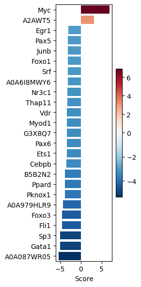
dc.pl.barplot(
    data=tf_acts1,
    name="Leukemic_spontaneous.vs.Normal",
    top=25,
    figsize=(3, 6),
)

Contrast 2: Leukemic_SB vs Normal

mat2 = results_df2[["stat"]].T.rename(index={"stat": "Leukemic_SB.vs.Normal"})
mat2

ID	Itm2a	Sergef	Fam109a	Dhx9	Ssu72	Eif2b2	Mks1	Vps28	Setd6	Psma4	...	Cd37	Rag2	Itgb1bp2	Sec23ip	Gosr1	Ctsw	Ryk	Rhd	Pxmp4	Gm25500
Leukemic_SB.vs.Normal	2.963769	13.983566	2.884977	-0.24563	0.179011	5.428026	6.215017	3.262983	5.410293	4.873833	...	1.520396	-2.272855	-3.153128	-6.110922	1.6341	-2.816943	-6.764932	-9.004647	-1.571242	0.455914

1 rows × 13286 columns

tf_acts2, tf_pvals2 = dc.mt.ulm(data=mat2, net=collectri, verbose=True)
tf_acts2

	A0A087WPA7	A0A087WQ36	A0A087WR05	A0A087WSP5	A0A0A6YWE3	A0A0A6YWQ4	A0A0A6YXS3	A0A0G2JEM8	A0A0J9YTU7	A0A0J9YTW3	...	Zgpat	Zhx2	Zic1	Znf143	Znf148	Znf263	Znf354c	Znf382	Znf436	Znf76
Leukemic_SB.vs.Normal	-1.03892	-0.881134	-5.416913	0.317954	-0.179198	0.755719	0.235632	-0.68796	0.674024	-0.397479	...	-1.245498	1.207684	0.267398	-0.224013	-2.08245	-0.238626	1.961743	-1.454379	-1.668492	0.348216

1 rows × 530 columns

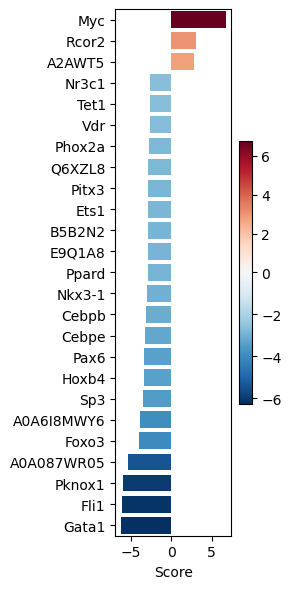
dc.pl.barplot(
    data=tf_acts2,
    name="Leukemic_SB.vs.Normal",
    top=25,
    figsize=(3, 6),
)

Retrieving potential receptors per condition

# We obtain ligand-receptor interactions from Omnipath, and we keep only the receptors
# This is our list of a prior potential receptors from which we will infer the network
unique_receptors = set(
    op.interactions.LigRecExtra.get(organisms="mouse", genesymbols=True)["target_genesymbol"].values.tolist()
)
len(unique_receptors)

849

Contrast 1: Leukemic_spontaneous vs Normal

def select_receptors(results_df, receptor_universe, graph, n=30, padj=0.05, min_log2fc=0.5):
    candidates = results_df.loc[results_df.index.intersection(receptor_universe)].copy()
    candidates = candidates.loc[
        (candidates["padj"] < padj) & (candidates["log2FoldChange"] >= min_log2fc)
    ]
    candidates = candidates.loc[candidates.index.intersection(graph.V)]
    return candidates.sort_values(["stat", "log2FoldChange"], ascending=False).head(n)


# The PKN is created below; receptor selection is finalized after that step.

Receptors are selected after constructing the PKN so that statistical evidence and PKN membership are both enforced.

Contrast 2: Leukemic_SB vs Normal

The same receptor rule is used for both conditions; no fixed top-\(n\) list is accepted without an evidence threshold.

This avoids treating weakly changing receptors as condition-specific inputs merely because they occupy a high rank.

Inferring intracellular signalling network with CORNETO

cn.info()

Installed version: v1.0.0rc5 Available backends: CVXPY v1.9.1 Default backend (corneto.opt): CVXPY Installed solvers: CLARABEL, SCS, GUROBI, SCIPY, HIGHS, OSQP Plot backend (default): auto -> graphviz Available plot backends: graphviz v0.21; graphviz-wasm Installed path: /docs/tutorials/contrib/multi_condition_tutorial/.pixi/envs/default/lib/python3.11/site-packages/corneto Repository: https://github.com/saezlab/corneto

from corneto.methods import CarnivalFlow

# CarnivalFlow.show_citations()

Setting prior knowledge graph

pkn = op.interactions.OmniPath.get(organisms="mouse", databases=["SIGNOR"], genesymbols=True)
pkn = pkn[pkn.consensus_direction == True]
pkn.head()

	source	target	source_genesymbol	target_genesymbol	is_directed	is_stimulation	is_inhibition	consensus_direction	consensus_stimulation	consensus_inhibition	curation_effort	references	sources	n_sources	n_primary_sources	n_references	references_stripped
0	P0C605	Q9QZC1	Prkg1	Trpc3	True	False	True	True	False	True	9	HPRD:14983059;KEA:14983059;ProtMapper:14983059...	HPRD;HPRD_KEA;HPRD_MIMP;KEA;MIMP;PhosphoPoint;...	15	8	2	14983059;16331690
1	P0C605	Q9WVC5	Prkg1	Trpc7	True	True	False	True	True	False	3	SIGNOR:21402151;TRIP:21402151;iPTMnet:21402151	SIGNOR;TRIP;iPTMnet	3	3	1	21402151
2	Q8K2C7	Q9EPK8	Os9	Trpv4	True	True	True	True	True	True	3	HPRD:17932042;SIGNOR:17932042;TRIP:17932042	HPRD;SIGNOR;TRIP	3	3	1	17932042
3	P35821	Q91WD2	Ptpn1	Trpv6	True	False	True	True	False	True	11	DEPOD:15894168;DEPOD:17197020;HPRD:15894168;In...	DEPOD;HPRD;IntAct;Lit-BM-17;SIGNOR;SPIKE_LC;TRIP	7	6	2	15894168;17197020
4	P68040	Q8CIR4	Rack1	Trpm6	True	False	True	True	False	True	2	SIGNOR:18258429;TRIP:18258429	SIGNOR;TRIP	2	2	1	18258429

pkn["interaction"] = pkn["is_stimulation"].astype(int) - pkn["is_inhibition"].astype(int)
sel_pkn = pkn[["source_genesymbol", "interaction", "target_genesymbol"]]
sel_pkn.head()

	source_genesymbol	interaction	target_genesymbol
0	Prkg1	-1	Trpc3
1	Prkg1	1	Trpc7
2	Os9	0	Trpv4
3	Ptpn1	-1	Trpv6
4	Rack1	-1	Trpm6

# We create the CORNETO graph by importing the edges and interaction
G = cn.Graph.from_sif_tuples([(r[0], r[1], r[2]) for _, r in sel_pkn.iterrows() if r[1] != 0])
G.shape  # nodes, edges

(4304, 9505)

Independent pathway view for held-out validation

Individual protein activity need not follow expression of the corresponding gene. We therefore use two unsigned validation views: whether selected internal-node genes are disproportionately deregulated, and whether the selected internal nodes concentrate in pathways that are deregulated as groups. SignaLink pathway annotations are used for the latter. They are not included in the CARNIVAL objective.

The installed resource currently exposes human symbols. Conserved symbols are mapped case-insensitively to mouse genes present in this dataset and PKN, and mapping coverage is reported explicitly.

signalink_human = dc.op.resource("SignaLink_pathway", organism="human")
mouse_symbol_lookup = {str(symbol).upper(): str(symbol) for symbol in G.V}
mouse_symbol_lookup.update(
    {str(symbol).upper(): str(symbol) for symbol in adata.var_names}
)

signalink = signalink_human.assign(
    genesymbol=signalink_human["genesymbol"].str.upper().map(mouse_symbol_lookup)
).dropna(subset=["genesymbol"])[["genesymbol", "pathway"]]
signalink = signalink.drop_duplicates()
pathway_net = signalink.rename(
    columns={"pathway": "source", "genesymbol": "target"}
).assign(weight=1.0)

pathway_members = {
    pathway: set(frame["genesymbol"])
    for pathway, frame in signalink.groupby("pathway")
}

def heldout_pathway_activity(results_df, contrast_name):
    matrix = results_df[["stat"]].T.rename(index={"stat": contrast_name})
    activities, _ = dc.mt.ulm(data=matrix, net=pathway_net, tmin=5, verbose=False)
    return activities.iloc[0].abs()


validation_pathways1 = heldout_pathway_activity(
    validation_results_df1, "Leukemic_spontaneous.vs.Normal"
)
validation_pathways2 = heldout_pathway_activity(
    validation_results_df2, "Leukemic_SB.vs.Normal"
)

pd.Series(
    {
        "human_annotation_genes": signalink_human["genesymbol"].nunique(),
        "mapped_mouse_genes": signalink["genesymbol"].nunique(),
        "mapped_pathways": signalink["pathway"].nunique(),
    },
    name="pathway_resource",
)

human_annotation_genes    1938
mapped_mouse_genes         816
mapped_pathways             13
Name: pathway_resource, dtype: int64

Identifying target TFs per condition

max_pval = 0.01

Contrast 1: Leukemic_spontaneous vs Normal

# As measurements, we take the estimated TFs, we will filter out TFs with p-val > 0.01
significant_tfs1 = (
    tf_acts1[tf_pvals1 <= max_pval].T.dropna().sort_values(by="Leukemic_spontaneous.vs.Normal", ascending=False)
)
significant_tfs1.head()

	Leukemic_spontaneous.vs.Normal
Myc	6.919333
B5B2N2	-3.745155
Ppard	-3.772645
Pknox1	-3.841270
A0A979HLR9	-4.223345

# We keep only the ones in the PKN graph
measurements1 = significant_tfs1.loc[significant_tfs1.index.intersection(G.V)].to_dict()[
    "Leukemic_spontaneous.vs.Normal"
]
measurements1

{'Myc': 6.919332774298009,
 'Ppard': -3.7726452616087784,
 'Pknox1': -3.841269863918438,
 'Foxo3': -4.4365678956436305,
 'Fli1': -4.488422107569552,
 'Sp3': -4.919151910048148,
 'Gata1': -4.936540966143217}

Contrast 2: Leukemic_SB vs Normal

# As measurements, we take the estimated TFs, we will filter out TFs with p-val > 0.01
significant_tfs2 = tf_acts2[tf_pvals2 <= max_pval].T.dropna().sort_values(by="Leukemic_SB.vs.Normal", ascending=False)
significant_tfs2.head()

	Leukemic_SB.vs.Normal
Myc	6.785773
A0A6I8MWY6	-3.894287
Foxo3	-3.979161
A0A087WR05	-5.416913
Pknox1	-6.016046

# We keep only the ones in the PKN graph
measurements2 = significant_tfs2.loc[significant_tfs2.index.intersection(G.V)].to_dict()["Leukemic_SB.vs.Normal"]
measurements2

{'Myc': 6.785773233182686,
 'Foxo3': -3.9791614216864715,
 'Pknox1': -6.01604625567456,
 'Fli1': -6.153183562598498,
 'Gata1': -6.283017534496937}

Comparable condition evidence

The conditions contain different numbers of significant TFs. Truncating the larger dictionary loses information, and the previous helper also changed the order of the conditions when the first dictionary was larger. Instead, all TFs are retained and their absolute weights are normalized to sum to one within each condition. This makes the maximum inactive-output cost comparable without changing CORNETO’s regularizer.

def normalized_signed_measurements(measurements):
    clean = {k: float(v) for k, v in measurements.items() if np.isfinite(v) and v != 0}
    total_weight = sum(abs(v) for v in clean.values())
    if total_weight == 0:
        raise ValueError("A condition has no non-zero TF measurements")
    return {k: v / total_weight for k, v in clean.items()}


d_measurements1 = normalized_signed_measurements(measurements1)
d_measurements2 = normalized_signed_measurements(measurements2)

assert set(d_measurements1) == set(measurements1)
assert set(d_measurements2) == set(measurements2)
assert np.isclose(sum(abs(v) for v in d_measurements1.values()), 1)
assert np.isclose(sum(abs(v) for v in d_measurements2.values()), 1)

measurement_summary = pd.DataFrame(
    {
        "condition": ["Leukemic_spontaneous", "Leukemic_SB"],
        "n_tfs": [len(d_measurements1), len(d_measurements2)],
        "total_weight": [
            sum(abs(v) for v in d_measurements1.values()),
            sum(abs(v) for v in d_measurements2.values()),
        ],
    }
)
measurement_summary

	condition	n_tfs	total_weight
0	Leukemic_spontaneous	7	1.0
1	Leukemic_SB	5	1.0

Condition-specific receptor inputs

Receptor expression is only a proxy for receptor activity, so candidates must show positive differential expression, pass the adjusted-\(p\) threshold, and occur in the PKN. Input signs remain unknown (0), as CORNETO infers their direction.

df_top_receptors1 = select_receptors(results_df1, unique_receptors, G)
df_top_receptors2 = select_receptors(results_df2, unique_receptors, G)

inputs1 = {k: 0 for k in df_top_receptors1.index}
inputs2 = {k: 0 for k in df_top_receptors2.index}

if not inputs1 or not inputs2:
    raise ValueError("Receptor filtering left a condition without candidate inputs")


def restrict_to_reachable_evidence(graph, inputs, measurements):
    condition_graph = graph.prune(list(inputs), list(measurements))
    retained_vertices = set(condition_graph.V)
    reachable_inputs = {node: value for node, value in inputs.items() if node in retained_vertices}
    reachable_measurements = {
        node: value for node, value in measurements.items() if node in retained_vertices
    }
    if not reachable_inputs or not reachable_measurements:
        raise ValueError("A condition has no receptor-to-TF path in the PKN")
    return reachable_inputs, normalized_signed_measurements(reachable_measurements)


inputs1, d_measurements1 = restrict_to_reachable_evidence(G, inputs1, d_measurements1)
inputs2, d_measurements2 = restrict_to_reachable_evidence(G, inputs2, d_measurements2)

pd.DataFrame(
    {
        "condition": ["Leukemic_spontaneous", "Leukemic_SB"],
        "n_receptors": [len(inputs1), len(inputs2)],
        "n_reachable_tfs": [len(d_measurements1), len(d_measurements2)],
        "reachable_tf_weight": [
            sum(abs(value) for value in d_measurements1.values()),
            sum(abs(value) for value in d_measurements2.values()),
        ],
        "receptors": [sorted(inputs1), sorted(inputs2)],
    }
)

	condition	n_receptors	n_reachable_tfs	reachable_tf_weight	receptors
0	Leukemic_spontaneous	14	6	1.0	[Acvr2b, Bambi, Cdon, Flt3, Galr3, Ifngr1, Ifn...
1	Leukemic_SB	12	4	1.0	[Acvr2b, Cdon, Fgfr1, Flt3, Galr3, Ifngr1, Ifn...

def make_carnival_sample(inputs, measurements):
    sample = {
        node: dict(value=value, role="input", mapping="vertex")
        for node, value in inputs.items()
    }
    sample.update(
        {
            node: dict(value=value, role="output", mapping="vertex")
            for node, value in measurements.items()
        }
    )
    return sample


carnival_data1 = make_carnival_sample(inputs1, d_measurements1)
carnival_data2 = make_carnival_sample(inputs2, d_measurements2)

data1 = cn.Data.from_cdict({"spontaneous": carnival_data1})
data2 = cn.Data.from_cdict({"SB": carnival_data2})
data = cn.Data.from_cdict(
    {"spontaneous": carnival_data1, "SB": carnival_data2}
)
data

Data(n_samples=2, n_feats=[20 16])

CARNIVAL solution and validation helpers

The same solver settings and diagnostics are used for the direct and multi-condition models. Keeping these definitions shared makes their fits and complexities comparable.

from corneto.methods import CarnivalFlow


def as_matrix(values):
    values = np.asarray(values)
    return values[:, None] if values.ndim == 1 else values


def solve_carnival(graph, dataset, lambda_reg):
    method = CarnivalFlow(lambda_reg=lambda_reg, indirect_rule_penalty=1)
    problem = method.build_from_data(graph, dataset)
    problem.solve(
        solver="GUROBI",
        verbosity=0,
        max_seconds=max_time,
        mip_gap=0.001,
        seed=seed,
        Threads=1,
    )
    return {
        "method": method,
        "problem": problem,
        "vertices": list(method.processed_graph.V),
        "vertex_value": as_matrix(problem.expr.vertex_value.value),
        "edge_value": as_matrix(problem.expr.edge_value.value),
        "objectives": {
            objective.name: float(np.asarray(objective.value).sum())
            for objective in problem.objectives
        },
    }


def tf_fit_metrics(solution, condition_index, measurements):
    positions = {node: i for i, node in enumerate(solution["vertices"])}
    reachable = {node: value for node, value in measurements.items() if node in positions}
    total = sum(abs(value) for value in reachable.values())
    if total == 0:
        return dict(reachable_tfs=0, reachable_weight=0, tf_match=0, tf_inactive=1, tf_opposite=0)

    matched = inactive = opposite = 0.0
    for node, expected in reachable.items():
        weight = abs(expected)
        observed = np.sign(solution["vertex_value"][positions[node], condition_index])
        if observed == np.sign(expected):
            matched += weight
        elif observed == 0:
            inactive += weight
        else:
            opposite += weight

    return dict(
        reachable_tfs=len(reachable),
        reachable_weight=total,
        tf_match=matched / total,
        tf_inactive=inactive / total,
        tf_opposite=opposite / total,
    )


def hypergeometric_z(population, positives, draws, hits):
    if population <= 1 or positives <= 0 or draws <= 0 or positives >= population:
        return 0.0
    rate = positives / population
    variance = draws * rate * (1 - rate) * (population - draws) / (population - 1)
    return (hits - draws * rate) / np.sqrt(variance) if variance > 0 else 0.0


def internal_validation_metrics(
    solution,
    condition_index,
    inputs,
    measurements,
    results_df,
    pathway_activity,
    min_abs_log2fc=0.5,
    max_padj=0.1,
):
    excluded = set(inputs) | set(measurements)
    values = pd.Series(
        solution["vertex_value"][:, condition_index], index=solution["vertices"]
    )
    active = values.loc[values.abs() > 0.5].drop(index=excluded, errors="ignore")

    background = results_df.index.intersection(solution["vertices"]).difference(excluded)
    evidence = results_df.loc[background, ["log2FoldChange", "padj"]].dropna()
    background = evidence.index
    active = active.loc[active.index.intersection(background)]
    deregulated = evidence.index[
        (evidence["log2FoldChange"].abs() >= min_abs_log2fc)
        & (evidence["padj"] <= max_padj)
    ]
    hits = active.index.intersection(deregulated)

    population = len(background)
    positives = len(deregulated)
    draws = len(active)
    n_hits = len(hits)
    selected_rate = n_hits / draws if draws else 0.0
    background_rate = positives / population if population else 0.0
    fold_enrichment = selected_rate / background_rate if background_rate else 0.0

    network_pathway_profile = {}
    annotated_active = set()
    background_set = set(background)
    active_set = set(active.index)
    for pathway, members in pathway_members.items():
        members = members & background_set
        if len(members) < 5:
            continue
        overlap = active_set & members
        annotated_active.update(overlap)
        network_pathway_profile[pathway] = max(
            0.0,
            hypergeometric_z(population, len(members), draws, len(overlap)),
        )

    network_pathway_profile = pd.Series(network_pathway_profile, dtype=float)
    common_pathways = network_pathway_profile.index.intersection(pathway_activity.index)
    network_scores = network_pathway_profile.loc[common_pathways].to_numpy()
    expression_scores = pathway_activity.loc[common_pathways].to_numpy()
    denominator = np.linalg.norm(network_scores) * np.linalg.norm(expression_scores)
    pathway_concordance = (
        float(network_scores @ expression_scores / denominator) if denominator else 0.0
    )

    return dict(
        active_internal_nodes=draws,
        deregulated_internal_nodes=n_hits,
        node_deregulated_fraction=selected_rate,
        background_deregulated_fraction=background_rate,
        node_deregulation_enrichment=fold_enrichment,
        node_deregulation_z=hypergeometric_z(
            population, positives, draws, n_hits
        ),
        annotated_internal_nodes=len(annotated_active),
        pathway_concordance=pathway_concordance,
    )


def structural_metrics(solution, condition_index, inputs):
    edge_values = solution["edge_value"][:, condition_index]
    vertex_values = solution["vertex_value"][:, condition_index]
    positions = {node: i for i, node in enumerate(solution["vertices"])}
    active_inputs = sum(
        node in positions and abs(vertex_values[positions[node]]) > 0.5 for node in inputs
    )
    return dict(
        active_edges=int(np.sum(np.abs(edge_values) > 0.5)),
        active_nodes=int(np.sum(np.abs(vertex_values) > 0.5)),
        active_inputs=int(active_inputs),
    )

Direct differential network: spontaneous leukemia vs SB leukemia

The two disease-versus-normal contrasts describe large shared leukemia effects. To ask what differs between leukemias, we must fit the direct contrast from the counts. We use Leukemic_spontaneous - Leukemic_SB, so positive values mean relatively higher in spontaneous leukemia and negative values mean relatively higher in SB leukemia. They do not mean absolute activation or inhibition relative to normal.

The training samples define genes, receptor candidates, TF activities, and the CARNIVAL network. The held-out leukemia samples are used only to select the differential-network lambda. The full data are used once at the end to refit the displayed network.

def fit_direct_de(adata_subset, min_prop=0.8, refit_cooks=True):
    direct = adata_subset.copy()
    dc.pp.filter_by_expr(
        direct,
        group="condition",
        min_count=10,
        min_total_count=15,
        large_n=10,
        min_prop=min_prop,
    )
    inference = DefaultInference()
    dds = DeseqDataSet(
        adata=direct,
        design="~condition",
        refit_cooks=refit_cooks,
        inference=inference,
        quiet=True,
    )
    dds.deseq2()
    stats = DeseqStats(
        dds,
        contrast=["condition", "Leukemic_spontaneous", "Leukemic_SB"],
        inference=inference,
        quiet=True,
    )
    stats.summary()
    return stats.results_df


direct_train_adata = adata[list(spontaneous_train) + list(sb_train)].copy()
direct_validation_adata = adata[
    list(spontaneous_validation) + list(sb_validation)
].copy()

direct_results = fit_direct_de(direct_train_adata)
direct_validation_results = fit_direct_de(
    direct_validation_adata, min_prop=0.5, refit_cooks=False
)
direct_results.sort_values("padj").head()

	baseMean	log2FoldChange	lfcSE	stat	pvalue	padj
ID
Nov	6726.372248	-10.171070	1.226824	-8.290569	1.127082e-16	1.509500e-12
Tuba1c	6612.117489	-1.100940	0.182744	-6.024495	1.696380e-09	1.135981e-05
Zfp874a	494.573758	0.736557	0.133421	5.520532	3.379756e-08	1.131627e-04
Nlrp1b	152.286506	2.714449	0.491272	5.525343	3.288427e-08	1.131627e-04
AI506816	1284.533981	-1.303951	0.244834	-5.325856	1.004785e-07	2.691416e-04

Gene-expression specificity

The left panel shows why the direct contrast is needed: most disease-versus-normal fold changes lie near the diagonal. Threshold-only categories are useful descriptions, but failure to cross a threshold in one contrast is not evidence that two leukemias differ. The right panel therefore uses the direct statistical test for specificity.

import matplotlib.pyplot as plt


gene_threshold = 0.5
gene_fdr = 0.05
common_genes = results_df1.index.intersection(results_df2.index)
control_comparison = pd.DataFrame(
    {
        "spontaneous_log2fc": results_df1.loc[common_genes, "log2FoldChange"],
        "spontaneous_padj": results_df1.loc[common_genes, "padj"],
        "SB_log2fc": results_df2.loc[common_genes, "log2FoldChange"],
        "SB_padj": results_df2.loc[common_genes, "padj"],
    }
).dropna()

spontaneous_sig = (
    (control_comparison["spontaneous_padj"] <= gene_fdr)
    & (control_comparison["spontaneous_log2fc"].abs() >= gene_threshold)
)
sb_sig = (
    (control_comparison["SB_padj"] <= gene_fdr)
    & (control_comparison["SB_log2fc"].abs() >= gene_threshold)
)
same_sign = np.sign(control_comparison["spontaneous_log2fc"]) == np.sign(
    control_comparison["SB_log2fc"]
)
control_comparison["category"] = "below threshold"
control_comparison.loc[spontaneous_sig & ~sb_sig, "category"] = "spontaneous only"
control_comparison.loc[~spontaneous_sig & sb_sig, "category"] = "SB only"
control_comparison.loc[spontaneous_sig & sb_sig & same_sign, "category"] = "shared, same sign"
control_comparison.loc[spontaneous_sig & sb_sig & ~same_sign, "category"] = "shared, opposite sign"

direct_gene_table = direct_results[["log2FoldChange", "padj"]].dropna().copy()
direct_gene_table["specificity"] = "not direct-DE"
direct_gene_sig = (
    (direct_gene_table["padj"] <= gene_fdr)
    & (direct_gene_table["log2FoldChange"].abs() >= gene_threshold)
)
direct_gene_table.loc[
    direct_gene_sig & (direct_gene_table["log2FoldChange"] > 0), "specificity"
] = "spontaneous higher"
direct_gene_table.loc[
    direct_gene_sig & (direct_gene_table["log2FoldChange"] < 0), "specificity"
] = "SB higher"

fig, axes = plt.subplots(1, 2, figsize=(12, 4.5))
category_colors = {
    "below threshold": "#d0d0d0",
    "shared, same sign": "#6f6f6f",
    "shared, opposite sign": "#8e44ad",
    "spontaneous only": "#d95f02",
    "SB only": "#1b9e77",
}
for category in category_colors:
    frame = control_comparison.loc[control_comparison["category"] == category]
    axes[0].scatter(
        frame["spontaneous_log2fc"],
        frame["SB_log2fc"],
        s=7,
        alpha=0.45,
        color=category_colors[category],
        label=f"{category} ({len(frame)})",
    )
limits = np.nanmax(
    np.abs(control_comparison[["spontaneous_log2fc", "SB_log2fc"]].to_numpy())
)
axes[0].plot([-limits, limits], [-limits, limits], "k--", linewidth=1)
axes[0].set(
    xlabel="Spontaneous vs normal log2FC",
    ylabel="SB vs normal log2FC",
    title="Control-relative effects",
)
axes[0].legend(fontsize=7, frameon=False)

volcano_colors = {
    "not direct-DE": "#d0d0d0",
    "spontaneous higher": "#d95f02",
    "SB higher": "#1b9e77",
}
volcano_y = -np.log10(direct_gene_table["padj"].clip(lower=1e-300))
for category in volcano_colors:
    mask = direct_gene_table["specificity"] == category
    axes[1].scatter(
        direct_gene_table.loc[mask, "log2FoldChange"],
        volcano_y.loc[mask],
        s=8,
        alpha=0.55,
        color=volcano_colors[category],
        label=f"{category} ({mask.sum()})",
    )
axes[1].axvline(-gene_threshold, color="black", linestyle="--", linewidth=0.8)
axes[1].axvline(gene_threshold, color="black", linestyle="--", linewidth=0.8)
axes[1].axhline(-np.log10(gene_fdr), color="black", linestyle="--", linewidth=0.8)
axes[1].set(
    xlabel="Spontaneous vs SB log2FC",
    ylabel="-log10 adjusted p-value",
    title="Direct leukemia contrast",
)
axes[1].legend(fontsize=8, frameon=False)
plt.tight_layout()
plt.show()

shared_de = spontaneous_sig & sb_sig
gene_specificity_metrics = pd.Series(
    {
        "control-relative log2FC Pearson r": control_comparison[
            ["spontaneous_log2fc", "SB_log2fc"]
        ].corr().iloc[0, 1],
        "spontaneous vs normal DE genes": int(spontaneous_sig.sum()),
        "SB vs normal DE genes": int(sb_sig.sum()),
        "shared DE genes": int(shared_de.sum()),
        "shared DE genes with same sign (%)": 100
        * float(same_sign.loc[shared_de].mean()),
        "direct DE: spontaneous higher": int(
            (direct_gene_table["specificity"] == "spontaneous higher").sum()
        ),
        "direct DE: SB higher": int(
            (direct_gene_table["specificity"] == "SB higher").sum()
        ),
    },
    name="training_split",
)
gene_specificity_metrics

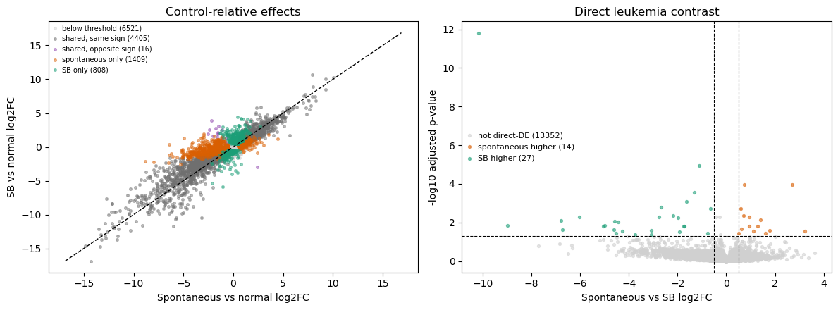
control-relative log2FC Pearson r        0.905318
spontaneous vs normal DE genes        5830.000000
SB vs normal DE genes                 5229.000000
shared DE genes                       4421.000000
shared DE genes with same sign (%)      99.638091
direct DE: spontaneous higher           14.000000
direct DE: SB higher                    27.000000
Name: training_split, dtype: float64

Receptor-expression and TF-activity specificity

Receptor expression is used only to nominate possible differential inputs; CARNIVAL is left to infer their signs. TF activities are inferred directly from the spontaneous-vs-SB gene-level statistic. The bars below retain direction: orange is relatively higher in spontaneous leukemia and green is relatively higher in SB leukemia.

def select_direct_receptors(
    results_df, receptor_universe, graph, n=30, padj=0.05, min_abs_log2fc=0.5
):
    candidates = results_df.loc[results_df.index.intersection(receptor_universe)].copy()
    candidates = candidates.loc[
        (candidates["padj"] <= padj)
        & (candidates["log2FoldChange"].abs() >= min_abs_log2fc)
    ]
    candidates = candidates.loc[candidates.index.intersection(graph.V)]
    return candidates.assign(abs_stat=candidates["stat"].abs()).sort_values(
        ["abs_stat", "padj"], ascending=[False, True]
    ).head(n)


direct_receptors = select_direct_receptors(direct_results, unique_receptors, G)
direct_mat = direct_results[["stat"]].T.rename(
    index={"stat": "Leukemic_spontaneous.vs.Leukemic_SB"}
)
direct_tf_acts, direct_tf_pvals = dc.mt.ulm(
    data=direct_mat, net=collectri, verbose=False
)
direct_significant_tfs = (
    direct_tf_acts[direct_tf_pvals <= max_pval]
    .T.dropna()
    .sort_values("Leukemic_spontaneous.vs.Leukemic_SB")
)

fig, axes = plt.subplots(1, 2, figsize=(12, 5))
receptor_plot = direct_receptors.sort_values("log2FoldChange")
axes[0].barh(
    receptor_plot.index,
    receptor_plot["log2FoldChange"],
    color=np.where(receptor_plot["log2FoldChange"] > 0, "#d95f02", "#1b9e77"),
)
axes[0].axvline(0, color="black", linewidth=0.8)
axes[0].set(
    xlabel="Direct contrast log2FC",
    title="Differentially expressed receptor candidates",
)

tf_plot = direct_significant_tfs.iloc[
    np.argsort(
        direct_significant_tfs[
            "Leukemic_spontaneous.vs.Leukemic_SB"
        ].abs().to_numpy()
    )[-20:]
].sort_values("Leukemic_spontaneous.vs.Leukemic_SB")
tf_values = tf_plot["Leukemic_spontaneous.vs.Leukemic_SB"]
axes[1].barh(
    tf_plot.index,
    tf_values,
    color=np.where(tf_values > 0, "#d95f02", "#1b9e77"),
)
axes[1].axvline(0, color="black", linewidth=0.8)
axes[1].set(xlabel="ULM activity score", title="Direct differential TF activities")
plt.tight_layout()
plt.show()

control_tf_common = tf_acts1.columns.intersection(tf_acts2.columns)
tf_profile_correlation = tf_acts1.loc[
    "Leukemic_spontaneous.vs.Normal", control_tf_common
].corr(tf_acts2.loc["Leukemic_SB.vs.Normal", control_tf_common])
control_tf_set1 = set(significant_tfs1.index)
control_tf_set2 = set(significant_tfs2.index)
control_receptor_set1 = set(df_top_receptors1.index)
control_receptor_set2 = set(df_top_receptors2.index)

receptor_tf_metrics = pd.DataFrame(
    {
        "feature": ["receptor candidates", "significant TF activities"],
        "spontaneous vs normal": [len(control_receptor_set1), len(control_tf_set1)],
        "SB vs normal": [len(control_receptor_set2), len(control_tf_set2)],
        "shared": [
            len(control_receptor_set1 & control_receptor_set2),
            len(control_tf_set1 & control_tf_set2),
        ],
        "control-relative Jaccard": [
            len(control_receptor_set1 & control_receptor_set2)
            / len(control_receptor_set1 | control_receptor_set2),
            len(control_tf_set1 & control_tf_set2)
            / len(control_tf_set1 | control_tf_set2),
        ],
        "direct: spontaneous higher": [
            int((direct_receptors["log2FoldChange"] > 0).sum()),
            int(
                (
                    direct_significant_tfs[
                        "Leukemic_spontaneous.vs.Leukemic_SB"
                    ]
                    > 0
                ).sum()
            ),
        ],
        "direct: SB higher": [
            int((direct_receptors["log2FoldChange"] < 0).sum()),
            int(
                (
                    direct_significant_tfs[
                        "Leukemic_spontaneous.vs.Leukemic_SB"
                    ]
                    < 0
                ).sum()
            ),
        ],
    }
).set_index("feature")

display(receptor_tf_metrics)
print(f"Control-relative TF activity Pearson r: {tf_profile_correlation:.3f}")

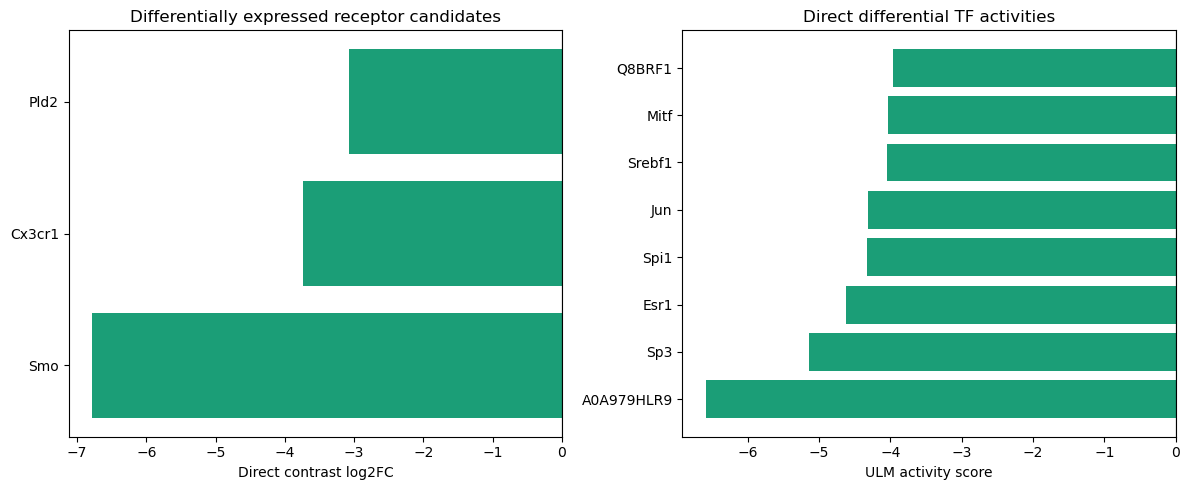
	spontaneous vs normal	SB vs normal	shared	control-relative Jaccard	direct: spontaneous higher	direct: SB higher
feature
receptor candidates	30	30	20	0.500000	0	3
significant TF activities	10	7	6	0.545455	0	8

Control-relative TF activity Pearson r: 0.854

Select lambda for the differential network

The direct network uses the same five-percentage-point TF-fit tolerance as the joint analysis. Among eligible lambdas, held-out deregulation of internal-node genes and held-out pathway concordance are weighted equally. We then choose the sparsest network within 0.05 of the best validation score. This selects complexity without using the samples that will be used for the final refit.

direct_measurements_raw = direct_significant_tfs.loc[
    direct_significant_tfs.index.intersection(G.V)
].to_dict()["Leukemic_spontaneous.vs.Leukemic_SB"]
direct_measurements = normalized_signed_measurements(direct_measurements_raw)
direct_inputs = {node: 0 for node in direct_receptors.index}
direct_inputs, direct_measurements = restrict_to_reachable_evidence(
    G, direct_inputs, direct_measurements
)
direct_sample = make_carnival_sample(direct_inputs, direct_measurements)
direct_data = cn.Data.from_cdict({"spontaneous_vs_SB": direct_sample})
direct_validation_pathways = heldout_pathway_activity(
    direct_validation_results, "Leukemic_spontaneous.vs.Leukemic_SB"
)

lambda_values = [0.0, 0.001, 0.003, 0.01, 0.03, 0.1, 0.3]
direct_solutions = {}
direct_rows = []
for lambda_reg in lambda_values:
    print(f"Solving direct contrast, lambda={lambda_reg:g}")
    solution = solve_carnival(G, direct_data, lambda_reg)
    direct_solutions[lambda_reg] = solution
    direct_rows.append(
        {
            "lambda": lambda_reg,
            **tf_fit_metrics(solution, 0, direct_measurements),
            **internal_validation_metrics(
                solution,
                0,
                direct_inputs,
                direct_measurements,
                direct_validation_results,
                direct_validation_pathways,
            ),
            **structural_metrics(solution, 0, direct_inputs),
        }
    )

direct_diagnostics = pd.DataFrame(direct_rows).set_index("lambda")
direct_baseline_match = direct_diagnostics.loc[0.0, "tf_match"]
direct_diagnostics["eligible"] = (
    (direct_diagnostics["tf_match"] >= direct_baseline_match - 0.05)
    & (direct_diagnostics["active_edges"] > 0)
    & (direct_diagnostics["active_inputs"] > 0)
)
positive_direct_node_z = direct_diagnostics["node_deregulation_z"].clip(lower=0)
best_direct_node_z = positive_direct_node_z.max()
best_direct_pathway = direct_diagnostics["pathway_concordance"].max()
direct_diagnostics["relative_node_validation"] = (
    positive_direct_node_z / best_direct_node_z if best_direct_node_z > 0 else 0.0
)
direct_diagnostics["relative_pathway_validation"] = (
    direct_diagnostics["pathway_concordance"] / best_direct_pathway
    if best_direct_pathway > 0
    else 0.0
)
direct_diagnostics["validation_score"] = direct_diagnostics[
    ["relative_node_validation", "relative_pathway_validation"]
].mean(axis=1)

eligible_direct = direct_diagnostics.loc[direct_diagnostics["eligible"]]
if eligible_direct.empty:
    raise RuntimeError("No lambda preserves a fitted, non-empty differential network")
best_direct_validation = eligible_direct["validation_score"].max()
near_best_direct = eligible_direct.loc[
    eligible_direct["validation_score"] >= best_direct_validation - 0.05
]
selected_direct_lambda = (
    near_best_direct.reset_index()
    .sort_values(
        ["active_edges", "validation_score", "lambda"],
        ascending=[True, False, False],
    )
    .iloc[0]["lambda"]
)

fig, axis = plt.subplots(figsize=(7, 4))
axis.plot(
    direct_diagnostics.index,
    direct_diagnostics["tf_match"],
    marker="o",
    label="TF matched weight",
)
axis.plot(
    direct_diagnostics.index,
    direct_diagnostics["validation_score"],
    marker="o",
    label="held-out validation",
)
axis.axvline(selected_direct_lambda, color="black", linestyle="--", label="selected lambda")
axis.set(xscale="symlog", xlabel="lambda", ylabel="score", ylim=(-0.03, 1.03))
axis.legend(frameon=False)
axis.set_title("Differential-network model selection")
plt.tight_layout()
plt.show()

display(direct_diagnostics)
print(f"Selected differential-network lambda: {selected_direct_lambda:g}")

Solving direct contrast, lambda=0
Unreachable vertices for sample: 0
Set parameter Username
Set parameter LicenseID to value 2775543
Academic license - for non-commercial use only - expires 2027-02-05
Solving direct contrast, lambda=0.001
Unreachable vertices for sample: 0
Solving direct contrast, lambda=0.003
Unreachable vertices for sample: 0
Solving direct contrast, lambda=0.01
Unreachable vertices for sample: 0
Solving direct contrast, lambda=0.03
Unreachable vertices for sample: 0
Solving direct contrast, lambda=0.1
Unreachable vertices for sample: 0
Solving direct contrast, lambda=0.3
Unreachable vertices for sample: 0
Selected differential-network lambda: 0.03

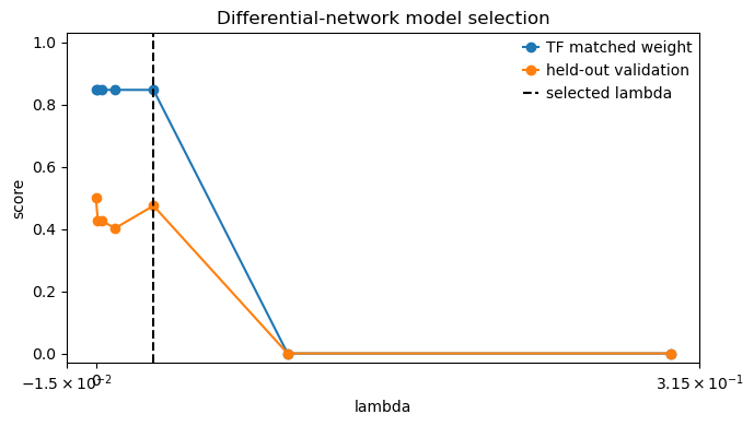
	reachable_tfs	reachable_weight	tf_match	tf_inactive	tf_opposite	active_internal_nodes	deregulated_internal_nodes	node_deregulated_fraction	background_deregulated_fraction	node_deregulation_enrichment	node_deregulation_z	annotated_internal_nodes	pathway_concordance	active_edges	active_nodes	active_inputs	eligible	relative_node_validation	relative_pathway_validation	validation_score
lambda
0.000	6	1.0	0.84753	0.15247	0.0	13	0	0.0	0.006791	0.0	-0.301232	10	0.744590	19	19	1	True	0.0	1.000000	0.500000
0.001	6	1.0	0.84753	0.15247	0.0	11	0	0.0	0.006791	0.0	-0.276613	10	0.634779	17	17	1	True	0.0	0.852522	0.426261
0.003	6	1.0	0.84753	0.15247	0.0	11	0	0.0	0.006791	0.0	-0.276613	10	0.634779	17	17	1	True	0.0	0.852522	0.426261
0.010	6	1.0	0.84753	0.15247	0.0	11	0	0.0	0.006791	0.0	-0.276613	9	0.599674	17	17	1	True	0.0	0.805375	0.402688
0.030	6	1.0	0.84753	0.15247	0.0	11	0	0.0	0.006791	0.0	-0.276613	9	0.707311	17	17	1	True	0.0	0.949933	0.474966
0.100	6	1.0	0.00000	1.00000	0.0	0	0	0.0	0.006791	0.0	0.000000	0	0.000000	0	0	0	False	0.0	0.000000	0.000000
0.300	6	1.0	0.00000	1.00000	0.0	0	0	0.0	0.006791	0.0	0.000000	0	0.000000	0	0	0	False	0.0	0.000000	0.000000

Selected differential network and full-data corroboration

The selected training network remains the inferential result: it was frozen before the held-out samples were used for validation. Rebuilding the topology after adding those samples would consume the holdout and, because CARNIVAL’s edge penalty is absolute, the same lambda is not automatically comparable when many more significant TF outputs enter the full-data contrast.

We therefore use all leukemia samples only for a sensitivity summary of gene, receptor, and TF evidence. The network shown below is the held-out-tested model. Its node signs are relative: +1 means higher inferred activity in spontaneous leukemia and -1 means higher inferred activity in SB leukemia.

full_direct_adata = adata[
    adata.obs["condition"].isin(["Leukemic_spontaneous", "Leukemic_SB"])
].copy()
full_direct_results = fit_direct_de(full_direct_adata)
full_direct_mat = full_direct_results[["stat"]].T.rename(
    index={"stat": "Leukemic_spontaneous.vs.Leukemic_SB"}
)
full_direct_tf_acts, full_direct_tf_pvals = dc.mt.ulm(
    data=full_direct_mat, net=collectri, verbose=False
)
full_direct_significant_tfs = (
    full_direct_tf_acts[full_direct_tf_pvals <= max_pval].T.dropna()
)
full_direct_receptors = select_direct_receptors(
    full_direct_results, unique_receptors, G
)

full_direct_gene_mask = (
    (full_direct_results["padj"] <= gene_fdr)
    & (full_direct_results["log2FoldChange"].abs() >= gene_threshold)
)
full_direct_gene_sign = np.sign(
    full_direct_results.loc[full_direct_gene_mask, "log2FoldChange"]
)
training_specific_genes = direct_gene_table.index[direct_gene_sig]
replicated_genes = training_specific_genes.intersection(full_direct_gene_sign.index)
training_full_sign_agreement = (
    np.sign(direct_results.loc[replicated_genes, "log2FoldChange"])
    == full_direct_gene_sign.loc[replicated_genes]
).mean()

final_direct_solution = direct_solutions[selected_direct_lambda]
selected_direct_metrics = pd.Series(
    {
        **tf_fit_metrics(final_direct_solution, 0, direct_measurements),
        **structural_metrics(final_direct_solution, 0, direct_inputs),
        "heldout_validation_score": direct_diagnostics.loc[
            selected_direct_lambda, "validation_score"
        ],
        "heldout_pathway_concordance": direct_diagnostics.loc[
            selected_direct_lambda, "pathway_concordance"
        ],
    },
    name="held-out-tested differential network",
)
full_evidence_metrics = pd.Series(
    {
        "direct_DE_genes": int(full_direct_gene_mask.sum()),
        "spontaneous_higher_genes": int((full_direct_gene_sign > 0).sum()),
        "SB_higher_genes": int((full_direct_gene_sign < 0).sum()),
        "differential_receptor_candidates": len(full_direct_receptors),
        "significant_differential_TFs": len(full_direct_significant_tfs),
        "training_DE_genes_replicated": len(replicated_genes),
        "replicated_gene_direction_agreement": training_full_sign_agreement,
    },
    name="all-sample evidence sensitivity",
)

display(selected_direct_metrics)
full_evidence_metrics

reachable_tfs                   6.000000
reachable_weight                1.000000
tf_match                        0.847530
tf_inactive                     0.152470
tf_opposite                     0.000000
active_edges                   17.000000
active_nodes                   17.000000
active_inputs                   1.000000
heldout_validation_score        0.474966
heldout_pathway_concordance     0.707311
Name: held-out-tested differential network, dtype: float64

direct_DE_genes                        537.0
spontaneous_higher_genes                58.0
SB_higher_genes                        479.0
differential_receptor_candidates        30.0
significant_differential_TFs            35.0
training_DE_genes_replicated            39.0
replicated_gene_direction_agreement      1.0
Name: all-sample evidence sensitivity, dtype: float64

direct_edge_values = final_direct_solution["edge_value"][:, 0]
direct_active_edges = np.flatnonzero(np.abs(direct_edge_values) > 0.5)
final_direct_graph = final_direct_solution["method"].processed_graph.edge_subgraph(
    direct_active_edges
)
full_vertex_positions = {
    node: i for i, node in enumerate(final_direct_solution["vertices"])
}
plot_vertex_values = np.array(
    [
        final_direct_solution["vertex_value"][full_vertex_positions[node], 0]
        for node in final_direct_graph.V
    ]
)
plot_edge_values = direct_edge_values[direct_active_edges]
direct_node_roles = {
    **{node: "input" for node in direct_inputs},
    **{node: "output" for node in direct_measurements},
}

final_direct_graph.plot(
    preset="signaling",
    data={
        "vertex_values": plot_vertex_values,
        "edge_values": plot_edge_values,
    },
    node_roles=direct_node_roles,
    layout="dot",
)

The direct network captures relative leukemia differences that the shared-control models are not forced to fit. It should therefore be interpreted alongside—not instead of—the multi-condition analysis below: the former emphasizes differences, while the latter retains mechanisms shared by both leukemias relative to normal.

Multi-condition network inference and deterministic \(\lambda\) analysis

We now return to the two disease-versus-normal conditions. These models retain shared leukemia biology and estimate absolute control-relative signs; their union regularizer is not intended to replace the direct differential network above.

lambda_values = [0.0, 0.001, 0.003, 0.01, 0.03, 0.1, 0.3]
condition_specs = {
    "spontaneous": dict(
        data=data1,
        inputs=inputs1,
        measurements=d_measurements1,
        results=validation_results_df1,
        pathway_activity=validation_pathways1,
    ),
    "SB": dict(
        data=data2,
        inputs=inputs2,
        measurements=d_measurements2,
        results=validation_results_df2,
        pathway_activity=validation_pathways2,
    ),
}

single_solutions = {}
joint_solutions = {}
diagnostic_rows = []

for lambda_reg in lambda_values:
    print(f"Solving lambda={lambda_reg:g}")
    single_solutions[lambda_reg] = {
        name: solve_carnival(G, spec["data"], lambda_reg)
        for name, spec in condition_specs.items()
    }
    joint_solutions[lambda_reg] = solve_carnival(G, data, lambda_reg)
    joint_edge_activity = np.abs(joint_solutions[lambda_reg]["edge_value"]) > 0.5
    union_edges = int(np.any(joint_edge_activity, axis=1).sum())
    shared_edges = int(np.all(joint_edge_activity, axis=1).sum())

    for condition_index, (name, spec) in enumerate(condition_specs.items()):
        single = single_solutions[lambda_reg][name]
        joint = joint_solutions[lambda_reg]
        single_fit = tf_fit_metrics(single, 0, spec["measurements"])
        joint_fit = tf_fit_metrics(joint, condition_index, spec["measurements"])
        row = {
            "lambda": lambda_reg,
            "condition": name,
            **joint_fit,
            **internal_validation_metrics(
                joint,
                condition_index,
                spec["inputs"],
                spec["measurements"],
                spec["results"],
                spec["pathway_activity"],
            ),
            **structural_metrics(joint, condition_index, spec["inputs"]),
            "single_tf_match": single_fit["tf_match"],
            "joint_fit_regret": max(0.0, single_fit["tf_match"] - joint_fit["tf_match"]),
            "union_edges": union_edges,
            "shared_edges": shared_edges,
        }
        diagnostic_rows.append(row)

diagnostics = pd.DataFrame(diagnostic_rows)
diagnostics

Solving lambda=0
Unreachable vertices for sample: 0
Unreachable vertices for sample: 0
Unreachable vertices for sample: 2
Unreachable vertices for sample: 10
Solving lambda=0.001
Unreachable vertices for sample: 0
Unreachable vertices for sample: 0
Unreachable vertices for sample: 2
Unreachable vertices for sample: 10
Solving lambda=0.003
Unreachable vertices for sample: 0
Unreachable vertices for sample: 0
Unreachable vertices for sample: 2
Unreachable vertices for sample: 10
Solving lambda=0.01
Unreachable vertices for sample: 0
Unreachable vertices for sample: 0
Unreachable vertices for sample: 2
Unreachable vertices for sample: 10
Solving lambda=0.03
Unreachable vertices for sample: 0
Unreachable vertices for sample: 0
Unreachable vertices for sample: 2
Unreachable vertices for sample: 10
Solving lambda=0.1
Unreachable vertices for sample: 0
Unreachable vertices for sample: 0
Unreachable vertices for sample: 2
Unreachable vertices for sample: 10
Solving lambda=0.3
Unreachable vertices for sample: 0
Unreachable vertices for sample: 0
Unreachable vertices for sample: 2
Unreachable vertices for sample: 10

	lambda	condition	reachable_tfs	reachable_weight	tf_match	tf_inactive	tf_opposite	active_internal_nodes	deregulated_internal_nodes	node_deregulated_fraction	...	node_deregulation_z	annotated_internal_nodes	pathway_concordance	active_edges	active_nodes	active_inputs	single_tf_match	joint_fit_regret	union_edges	shared_edges
0	0.000	spontaneous	6	1.0	0.704499	0.295501	0.0	21	7	0.333333	...	-0.760992	16	0.657710	30	30	3	0.704499	0.0	35	6
1	0.000	SB	4	1.0	0.729194	0.270806	0.0	4	1	0.250000	...	-0.076571	3	0.552921	11	11	2	0.729194	0.0	35	6
2	0.001	spontaneous	6	1.0	0.704499	0.295501	0.0	9	3	0.333333	...	-0.493077	9	0.788685	14	14	1	0.704499	0.0	14	10
3	0.001	SB	4	1.0	0.729194	0.270806	0.0	5	1	0.200000	...	-0.339298	5	0.727538	10	10	1	0.729194	0.0	14	10
4	0.003	spontaneous	6	1.0	0.704499	0.295501	0.0	8	2	0.250000	...	-0.945899	8	0.802111	14	14	1	0.704499	0.0	14	12
5	0.003	SB	4	1.0	0.729194	0.270806	0.0	7	1	0.142857	...	-0.745687	7	0.772395	12	12	1	0.729194	0.0	14	12
6	0.010	spontaneous	6	1.0	0.704499	0.295501	0.0	9	3	0.333333	...	-0.493077	9	0.788685	14	14	1	0.704499	0.0	14	10
7	0.010	SB	4	1.0	0.729194	0.270806	0.0	5	1	0.200000	...	-0.339298	5	0.727538	10	10	1	0.729194	0.0	14	10
8	0.030	spontaneous	6	1.0	0.704499	0.295501	0.0	9	3	0.333333	...	-0.493077	9	0.818096	14	14	1	0.704499	0.0	14	10
9	0.030	SB	4	1.0	0.729194	0.270806	0.0	5	1	0.200000	...	-0.339298	5	0.730120	10	10	1	0.729194	0.0	14	10
10	0.100	spontaneous	6	1.0	0.537594	0.462406	0.0	6	3	0.500000	...	0.430854	6	0.850635	10	10	1	0.000000	0.0	10	10
11	0.100	SB	4	1.0	0.729194	0.270806	0.0	5	1	0.200000	...	-0.339298	5	0.748767	10	10	1	0.000000	0.0	10	10
12	0.300	spontaneous	6	1.0	0.000000	1.000000	0.0	0	0	0.000000	...	0.000000	0	0.000000	0	0	0	0.000000	0.0	0	0
13	0.300	SB	4	1.0	0.000000	1.000000	0.0	0	0	0.000000	...	0.000000	0	0.000000	0	0	0	0.000000	0.0	0	0

14 rows × 22 columns

Eligibility and fair scoring

Because TF evidence is normalized to total weight one per condition, a five-percentage-point loss in matched TF weight is used as the admissibility tolerance. A candidate is rejected if either condition has no active input, edge, or matched TF, or if joint fitting loses more TF support than allowed relative to the joint \(\lambda=0\) and single-condition references. This keeps internal-network validation from rewarding sparsity obtained by discarding important outputs.

Eligible networks are scored using only held-out expression. The node score asks whether selected internal-node genes are more often deregulated than the reachable PKN background, without requiring expression and inferred protein activity to have the same sign. The pathway score compares SignaLink enrichment among selected internal nodes with absolute pathway-level deregulation in held-out expression. Both components are normalized within condition and weighted equally; the worst-condition score prevents the larger SB group from masking failure in the spontaneous condition.

baseline_match = (
    diagnostics.loc[diagnostics["lambda"] == 0]
    .set_index("condition")["tf_match"]
    .to_dict()
)
tf_tolerance = {"spontaneous": 0.05, "SB": 0.05}

diagnostics["fit_gate"] = diagnostics.apply(
    lambda row: row.tf_match >= baseline_match[row.condition] - tf_tolerance[row.condition],
    axis=1,
)
diagnostics["single_fit_gate"] = diagnostics.apply(
    lambda row: row.joint_fit_regret <= tf_tolerance[row.condition], axis=1
)
diagnostics["nonempty_gate"] = (
    (diagnostics["active_edges"] > 0)
    & (diagnostics["active_inputs"] > 0)
    & (diagnostics["tf_match"] > 0)
)
diagnostics["condition_eligible"] = (
    diagnostics["fit_gate"]
    & diagnostics["single_fit_gate"]
    & diagnostics["nonempty_gate"]
)

positive_node_z = diagnostics["node_deregulation_z"].clip(lower=0)
best_node_z = positive_node_z.groupby(diagnostics["condition"]).transform("max")
best_pathway = diagnostics.groupby("condition")["pathway_concordance"].transform("max")
diagnostics["relative_node_validation"] = np.divide(
    positive_node_z,
    best_node_z,
    out=np.zeros(len(diagnostics), dtype=float),
    where=best_node_z > 0,
)
diagnostics["relative_pathway_validation"] = np.divide(
    diagnostics["pathway_concordance"],
    best_pathway,
    out=np.zeros(len(diagnostics), dtype=float),
    where=best_pathway > 0,
)
diagnostics["validation_score"] = diagnostics[
    ["relative_node_validation", "relative_pathway_validation"]
].mean(axis=1)

selection = diagnostics.groupby("lambda").agg(
    eligible=("condition_eligible", "all"),
    fair_score=("validation_score", "min"),
    mean_score=("validation_score", "mean"),
    union_edges=("union_edges", "first"),
)

eligible = selection.loc[selection["eligible"]].copy()
if eligible.empty:
    raise RuntimeError("No lambda preserves a non-empty, adequately fitted network for both conditions")

best_fair = eligible["fair_score"].max()
near_best = eligible.loc[eligible["fair_score"] >= best_fair - 0.05]
selected_lambda = (
    near_best.reset_index()
    .sort_values(
        ["union_edges", "fair_score", "lambda"],
        ascending=[True, False, False],
    )
    .iloc[0]["lambda"]
)

display(selection)
print(f"Selected lambda: {selected_lambda:g}")
diagnostics.loc[diagnostics["lambda"] == selected_lambda]

	eligible	fair_score	mean_score	union_edges
lambda
0.000	True	0.357926	0.372263	35
0.001	True	0.463586	0.467274	14
0.003	True	0.471478	0.485739	14
0.010	True	0.463586	0.467274	14
0.030	True	0.472634	0.476754	14
0.100	False	0.484705	0.742352	10
0.300	False	0.000000	0.000000	0

Selected lambda: 0.03

	lambda	condition	reachable_tfs	reachable_weight	tf_match	tf_inactive	tf_opposite	active_internal_nodes	deregulated_internal_nodes	node_deregulated_fraction	...	joint_fit_regret	union_edges	shared_edges	fit_gate	single_fit_gate	nonempty_gate	condition_eligible	relative_node_validation	relative_pathway_validation	validation_score
8	0.03	spontaneous	6	1.0	0.704499	0.295501	0.0	9	3	0.333333	...	0.0	14	10	True	True	True	True	0.0	0.961747	0.480874
9	0.03	SB	4	1.0	0.729194	0.270806	0.0	5	1	0.200000	...	0.0	14	10	True	True	True	True	0.0	0.945267	0.472634

2 rows × 29 columns

Held-out validation interpretation

Lambda selection above uses a fixed stratified biological holdout. TFs, receptor inputs, and networks are inferred only from training samples. Held-out expression is used only to test whether selected internal-node genes are disproportionately deregulated and whether their pathway composition agrees with held-out pathway-level deregulation. Neither criterion assumes that a protein’s activity sign must equal the expression sign of its gene.

These criteria support transcriptional responsiveness of network regions, not direct validation of receptor, kinase, or protein activity. Because the spontaneous holdout is necessarily small, the scores are tutorial-scale model-selection evidence rather than precise generalization estimates. A production analysis should repeat the stratified split, use sample-level pathway activities, and aggregate paired condition scores and label-permutation controls.

This data-level holdout is distinct from alternative-network sampling: it informs model selection, whereas the solution sampler below is run only after lambda has been fixed.

Final model at the selected \(\lambda\)

def fit_full_de(adata_subset, disease_condition):
    full = adata_subset.copy()
    dc.pp.filter_by_expr(
        full,
        group="condition",
        min_count=10,
        min_total_count=15,
        large_n=10,
        min_prop=0.8,
    )
    inference = DefaultInference()
    dds = DeseqDataSet(
        adata=full,
        design="~condition",
        refit_cooks=True,
        inference=inference,
        quiet=True,
    )
    dds.deseq2()
    stats = DeseqStats(
        dds,
        contrast=["condition", disease_condition, "Normal"],
        inference=inference,
        quiet=True,
    )
    stats.summary()
    return stats.results_df


def infer_measurements(results_df, contrast_name):
    matrix = results_df[["stat"]].T.rename(index={"stat": contrast_name})
    activities, pvalues = dc.mt.ulm(data=matrix, net=collectri, verbose=False)
    selected = activities[pvalues <= max_pval].T.dropna()
    raw = selected.loc[selected.index.intersection(G.V)].to_dict()[contrast_name]
    return normalized_signed_measurements(raw)


full_adata1 = adata[adata.obs["condition"].isin(["Normal", "Leukemic_spontaneous"])].copy()
full_adata2 = adata[adata.obs["condition"].isin(["Normal", "Leukemic_SB"])].copy()
full_results_df1 = fit_full_de(full_adata1, "Leukemic_spontaneous")
full_results_df2 = fit_full_de(full_adata2, "Leukemic_SB")

final_measurements1 = infer_measurements(
    full_results_df1, "Leukemic_spontaneous.vs.Normal"
)
final_measurements2 = infer_measurements(full_results_df2, "Leukemic_SB.vs.Normal")
final_receptors1 = select_receptors(full_results_df1, unique_receptors, G)
final_receptors2 = select_receptors(full_results_df2, unique_receptors, G)
final_inputs1 = {node: 0 for node in final_receptors1.index}
final_inputs2 = {node: 0 for node in final_receptors2.index}
final_inputs1, final_measurements1 = restrict_to_reachable_evidence(
    G, final_inputs1, final_measurements1
)
final_inputs2, final_measurements2 = restrict_to_reachable_evidence(
    G, final_inputs2, final_measurements2
)

final_data = cn.Data.from_cdict(
    {
        "spontaneous": make_carnival_sample(final_inputs1, final_measurements1),
        "SB": make_carnival_sample(final_inputs2, final_measurements2),
    }
)
final_solution = solve_carnival(G, final_data, selected_lambda)

Unreachable vertices for sample: 3
Unreachable vertices for sample: 11

final_method = final_solution["method"]
final_problem = final_solution["problem"]

final_objectives = pd.Series(final_solution["objectives"], name="value")
final_objectives

error_spontaneous_0                   0.204626
penalty_indirect_rules_0              0.000000
error_SB_1                            0.343275
penalty_indirect_rules_1              0.000000
regularization_edge_has_signal_OR    14.000000
Name: value, dtype: float64

final_rows = []
for condition_index, (name, inputs, measurements) in enumerate(
    [
        ("spontaneous", final_inputs1, final_measurements1),
        ("SB", final_inputs2, final_measurements2),
    ]
):
    final_rows.append(
        {
            "condition": name,
            **tf_fit_metrics(final_solution, condition_index, measurements),
            **structural_metrics(final_solution, condition_index, inputs),
        }
    )

final_diagnostics = pd.DataFrame(final_rows).set_index("condition")
final_diagnostics

	reachable_tfs	reachable_weight	tf_match	tf_inactive	tf_opposite	active_edges	active_nodes	active_inputs
condition
spontaneous	5	1.0	0.795374	0.204626	0.0	14	14	1
SB	3	1.0	0.656725	0.343275	0.0	9	9	1

Alternative-solution sampling for the selected \(\lambda\)

Sampling is now a final robustness analysis and cannot influence \(\lambda\). Regularization is included in the near-optimality checks, the random generator is seeded, and acceptance counts are reported because max_samples is the number of attempts rather than a guaranteed number of returned networks.

from corneto.methods.sampler import sample_alternative_solutions


sampled = sample_alternative_solutions(
    final_problem,
    "edge_value",
    percentage=0.03,
    scale=max(float(selected_lambda) / 10, 1e-6),
    rel_opt_tol=0.05,
    max_samples=30,
    solver_kwargs=dict(
        solver="GUROBI", max_seconds=max_time, mip_gap=0.01, seed=seed, Threads=1
    ),
    rng=seed,
    collect_vars=["vertex_value", "edge_value"],
    exclude_objectives_pattern=None,
)

n_returned = len(sampled["vertex_value"])
print(f"Returned {n_returned} solutions: one incumbent plus {n_returned - 1} accepted perturbations")

Returned 31 solutions: one incumbent plus 30 accepted perturbations

vertex_frequency = np.mean(np.abs(sampled["vertex_value"]) > 0.5, axis=0)
edge_frequency = np.mean(np.abs(sampled["edge_value"]) > 0.5, axis=0)

vertex_frequency_df = pd.DataFrame(
    vertex_frequency,
    index=final_solution["vertices"],
    columns=["spontaneous", "SB"],
)
edge_frequency_df = pd.DataFrame(
    edge_frequency,
    index=final_method.processed_graph.E,
    columns=["spontaneous", "SB"],
)

sampling_summary = pd.DataFrame(
    {
        "condition": ["spontaneous", "SB"],
        "nodes_selected_at_least_50pct": (vertex_frequency_df >= 0.5).sum().to_numpy(),
        "nodes_selected_at_least_80pct": (vertex_frequency_df >= 0.8).sum().to_numpy(),
        "edges_selected_at_least_50pct": (edge_frequency_df >= 0.5).sum().to_numpy(),
        "edges_selected_at_least_80pct": (edge_frequency_df >= 0.8).sum().to_numpy(),
    }
)
sampling_summary

	condition	nodes_selected_at_least_50pct	nodes_selected_at_least_80pct	edges_selected_at_least_50pct	edges_selected_at_least_80pct
0	spontaneous	14	12	14	9
1	SB	9	7	9	4

The frequency tables distinguish stable conclusions from topology chosen arbitrarily among near-optimal solutions. If few edges recur, the result should be reported as structurally uncertain rather than using the samples to revisit \(\lambda\).