Knowledge-primed Neural Networks (KPNNs) for single cell data

In this tutorial we will show how CORNETO can be used to build custom neural network architectures informed by prior knowledge. We will see how to implement a knowledge-primed neural network¹. We will use the single cell data from the publication “Knowledge-primed neural networks enable biologically interpretable deep learning on single-cell sequencing data”, from Nikolaus Fortelny & Christoph Bock, where they used a single-cell RNA-seq dataset they previously generated², which measures cellular responses to T cell receptor (TCR) stimulation in a standardized in vitro model. The dataset was chosen due to the TCR signaling pathway’s complexity and its well-characterized role in orchestrating transcriptional responses to antigen detection in T cells.

Why CORNETO?

In the original publication, authors built a KPNN by searching on databases, building a Direct Acyclic Graph (DAG) by running shortest paths from TCR receptor to genes. However, this approach is not optimal. CORNETO, thanks to its advanced capabilities for modeling and optimization on networks, provides methods to automatically find DAG architectures in an optimal way.

In addition to this, CORNETO provides methods to build DAG NN architectures with ease using Keras +3, making KPNN implementation very flexible and interoperable with backends like Pytorch, Tensorflow and JAX.

How does it work?

Thanks to CORNETO’s building blocks for optimization over networks, we can easily model optimization problems to find DAG architectures from a Prior Knowledge Network. After we have the backbone, we can convert it to a neural network using the utility functions included in CORNETO.

References

1. Fortelny, N., & Bock, C. (2020). Knowledge-primed neural networks enable biologically interpretable deep learning on single-cell sequencing data. Genome biology, 21, 1-36.

2. Datlinger, P., Rendeiro, A. F., Schmidl, C., Krausgruber, T., Traxler, P., Klughammer, J., … & Bock, C. (2017). Pooled CRISPR screening with single-cell transcriptome readout. Nature methods, 14(3), 297-301.

Download and import the single cell dataset

import os
import tempfile
import urllib.parse
import urllib.request

import numpy as np
import pandas as pd
import scanpy as sc

import corneto as cn

with urllib.request.urlopen("http://kpnn.computational-epigenetics.org/") as response:
    web_input = response.geturl()
print("Effective URL:", web_input)

files = ["TCR_Edgelist.csv", "TCR_ClassLabels.csv", "TCR_Data.h5"]

temp_dir = tempfile.mkdtemp()

# Download files
file_paths = []
for file in files:
    url = urllib.parse.urljoin(web_input, file)
    output_path = os.path.join(temp_dir, file)
    print(f"Downloading {url} to {output_path}")
    try:
        with urllib.request.urlopen(url) as response:
            with open(output_path, "wb") as f:
                f.write(response.read())
        file_paths.append(output_path)
    except Exception as e:
        print(f"Failed to download {url}: {e}")

print("Downloaded files:")
for path in file_paths:
    print(path)

Effective URL: https://medical-epigenomics.org/papers/fortelny2019/
Downloading https://medical-epigenomics.org/papers/fortelny2019/TCR_Edgelist.csv to /var/folders/b4/gwkwsdb93sv11rtztqbm3l040000gn/T/tmpbv4ljrn2/TCR_Edgelist.csv
Downloading https://medical-epigenomics.org/papers/fortelny2019/TCR_ClassLabels.csv to /var/folders/b4/gwkwsdb93sv11rtztqbm3l040000gn/T/tmpbv4ljrn2/TCR_ClassLabels.csv
Downloading https://medical-epigenomics.org/papers/fortelny2019/TCR_Data.h5 to /var/folders/b4/gwkwsdb93sv11rtztqbm3l040000gn/T/tmpbv4ljrn2/TCR_Data.h5
Downloaded files:
/var/folders/b4/gwkwsdb93sv11rtztqbm3l040000gn/T/tmpbv4ljrn2/TCR_Edgelist.csv
/var/folders/b4/gwkwsdb93sv11rtztqbm3l040000gn/T/tmpbv4ljrn2/TCR_ClassLabels.csv
/var/folders/b4/gwkwsdb93sv11rtztqbm3l040000gn/T/tmpbv4ljrn2/TCR_Data.h5

# The data contains also the original network they built with shortest paths.
# We will use it to replicate the study
df_edges = pd.read_csv(file_paths[0])
df_labels = pd.read_csv(file_paths[1])
# Import the 10x data with Scanpy
adata = sc.read_10x_h5(file_paths[2])

df_labels

	barcode	TCR
0	AAACCTGCACACATGT-1	0
1	AAACCTGCACGTCTCT-1	0
2	AAACCTGTCAATACCG-1	0
3	AAACCTGTCGTGGTCG-1	0
4	AAACGGGTCTGAGTGT-1	0
...	...	...
1730	TTTCCTCGTCATGCCG-2	1
1731	TTTGCGCGTAGCCTCG-2	1
1732	TTTGGTTAGATACACA-2	1
1733	TTTGGTTGTATGAATG-2	1
1734	TTTGGTTTCCAAGTAC-2	1

1735 rows × 2 columns

df_edges

	parent	child
0	TCR	ZAP70
1	ZAP70	MAPK14
2	MAPK14	FOXO3
3	MAPK14	STAT1
4	MAPK14	STAT3
...	...	...
27574	HMGA1	MTRNR2L9_gene
27575	MYB	C12orf50_gene
27576	MYB	TRPC5OS_gene
27577	SOX2	TRPC5OS_gene
27578	CRTC1	MTRNR2L9_gene

27579 rows × 2 columns

adata.var

	gene_ids
DDX11L1	ENSG00000223972
WASH7P	ENSG00000227232
MIR6859-2	ENSG00000278267
MIR1302-10	ENSG00000243485
MIR1302-11	ENSG00000274890
...	...
Tcrlibrary_RUNX2_3_gene	Tcrlibrary_RUNX2_3_gene
Tcrlibrary_ZAP70_1_gene	Tcrlibrary_ZAP70_1_gene
Tcrlibrary_ZAP70_2_gene	Tcrlibrary_ZAP70_2_gene
Tcrlibrary_ZAP70_3_gene	Tcrlibrary_ZAP70_3_gene
Cas9_blast_gene	Cas9_blast_gene

64370 rows × 1 columns

# We can normalize the data, however, it is better to avoid
# preprocessing the whole dataset before splitting in training and test
# to avoid data leakage.
# NOTE: Normalization can be done inside the cross-val loop
# sc.pp.normalize_total(adata, target_sum=1e6)

# Log-transform the data does not leak data as it does not estimate anything
sc.pp.log1p(adata)

adata.obs

AAACCTGAGAAACCAT-1
AAACCTGAGAAACCGC-1
AAACCTGAGAAACCTA-1
AAACCTGAGAAACGAG-1
AAACCTGAGAAACGCC-1
...
TTTGTCATCTTTACAC-2
TTTGTCATCTTTACGT-2
TTTGTCATCTTTAGGG-2
TTTGTCATCTTTAGTC-2
TTTGTCATCTTTCCTC-2

1474560 rows × 0 columns

barcodes = adata.obs_names
barcodes

Index(['AAACCTGAGAAACCAT-1', 'AAACCTGAGAAACCGC-1', 'AAACCTGAGAAACCTA-1',
       'AAACCTGAGAAACGAG-1', 'AAACCTGAGAAACGCC-1', 'AAACCTGAGAAAGTGG-1',
       'AAACCTGAGAACAACT-1', 'AAACCTGAGAACAATC-1', 'AAACCTGAGAACTCGG-1',
       'AAACCTGAGAACTGTA-1',
       ...
       'TTTGTCATCTTGGGTA-2', 'TTTGTCATCTTGTACT-2', 'TTTGTCATCTTGTATC-2',
       'TTTGTCATCTTGTCAT-2', 'TTTGTCATCTTGTTTG-2', 'TTTGTCATCTTTACAC-2',
       'TTTGTCATCTTTACGT-2', 'TTTGTCATCTTTAGGG-2', 'TTTGTCATCTTTAGTC-2',
       'TTTGTCATCTTTCCTC-2'],
      dtype='object', length=1474560)

gene_names = adata.var.index
print(gene_names)

Index(['DDX11L1', 'WASH7P', 'MIR6859-2', 'MIR1302-10', 'MIR1302-11', 'FAM138A',
       'OR4G4P', 'OR4G11P', 'OR4F5', 'RP11-34P13.7',
       ...
       'Tcrlibrary_RUNX1_1_gene', 'Tcrlibrary_RUNX1_2_gene',
       'Tcrlibrary_RUNX1_3_gene', 'Tcrlibrary_RUNX2_1_gene',
       'Tcrlibrary_RUNX2_2_gene', 'Tcrlibrary_RUNX2_3_gene',
       'Tcrlibrary_ZAP70_1_gene', 'Tcrlibrary_ZAP70_2_gene',
       'Tcrlibrary_ZAP70_3_gene', 'Cas9_blast_gene'],
      dtype='object', length=64370)

len(set(df_labels.barcode.tolist()))

1735

len(set(barcodes.tolist()))

1474560

matched_barcodes = sorted(set(barcodes.tolist()) & set(df_labels.barcode.tolist()))
len(matched_barcodes)

1735

# This is the InPathsY data in the original code of KPNNs
df_labels

	barcode	TCR
0	AAACCTGCACACATGT-1	0
1	AAACCTGCACGTCTCT-1	0
2	AAACCTGTCAATACCG-1	0
3	AAACCTGTCGTGGTCG-1	0
4	AAACGGGTCTGAGTGT-1	0
...	...	...
1730	TTTCCTCGTCATGCCG-2	1
1731	TTTGCGCGTAGCCTCG-2	1
1732	TTTGGTTAGATACACA-2	1
1733	TTTGGTTGTATGAATG-2	1
1734	TTTGGTTTCCAAGTAC-2	1

1735 rows × 2 columns

Import PKN with CORNETO

cn.info()

Installed version: v1.0.0rc1 Available backends: CVXPY v1.7.5 Default backend (corneto.opt): CVXPY Installed solvers: CLARABEL, HIGHS, OSQP, SCIPY, SCS Plot backend (default): auto -> graphviz Available plot backends: graphviz v0.21; networkx v3.4.2+mpl v3.10.8; graphviz-wasm Installed path: /docs/tutorials/ml/.pixi/envs/default/lib/python3.11/site-packages/corneto Repository: https://github.com/saezlab/corneto

outputs_pkn = list(set(df_edges.parent.tolist()) - set(df_edges.child.tolist()))
inputs_pkn = set(df_edges.child.tolist()) - set(df_edges.parent.tolist())
input_pkn_genes = list(set(g.split("_")[0] for g in inputs_pkn))
len(inputs_pkn), len(outputs_pkn)

(13121, 1)

tuples = [(r.child, 1, r.parent) for _, r in df_edges.iterrows()]
G = cn.Graph.from_sif_tuples(tuples)
G = G.prune(inputs_pkn, outputs_pkn)

# Size of the original PKN provided by the authors
G.shape

(13439, 27579)

Select the single cell data for training

adata_matched = adata[adata.obs_names.isin(matched_barcodes), adata.var_names.isin(input_pkn_genes)]
adata_matched.shape

(1735, 14229)

non_zero_genes = set(adata_matched.to_df().columns[adata_matched.to_df().sum(axis=0) >= 1e-6].values)
len(non_zero_genes)

12459

len(non_zero_genes.intersection(adata_matched.var_names))

12459

adata_matched = adata_matched[:, adata_matched.var_names.isin(non_zero_genes)]
# Many duplicates still 0 counts
adata_matched = adata_matched[:, adata_matched.to_df().sum(axis=0) != 0]
adata_matched.shape

(1735, 12487)

df_expr = adata_matched.to_df()
df_expr = df_expr.groupby(df_expr.columns, axis=1).max()
df_expr

	A1BG	A2ML1	AAAS	AACS	AADAT	AAED1	AAGAB	AAK1	AAMDC	AAMP	...	ZSWIM8	ZUFSP	ZW10	ZWILCH	ZXDC	ZYG11A	ZYG11B	ZYX	ZZEF1	ZZZ3
AAACCTGCACACATGT-1	0.0	0.0	0.000000	0.693147	0.0	0.000000	0.000000	0.000000	0.0	1.098612	...	0.000000	0.000000	0.000000	0.000000	0.0	0.0	0.0	0.000000	0.000000	0.000000
AAACCTGCACGTCTCT-1	0.0	0.0	0.000000	0.000000	0.0	0.693147	0.000000	0.000000	0.0	0.693147	...	0.000000	0.000000	0.000000	0.000000	0.0	0.0	0.0	0.000000	0.000000	0.000000
AAACCTGTCAATACCG-1	0.0	0.0	0.000000	0.000000	0.0	0.000000	0.000000	0.000000	0.0	0.693147	...	0.000000	0.000000	0.000000	0.000000	0.0	0.0	0.0	0.000000	0.000000	0.000000
AAACCTGTCGTGGTCG-1	0.0	0.0	1.098612	0.000000	0.0	0.000000	0.000000	0.000000	0.0	1.098612	...	0.000000	0.693147	0.000000	0.693147	0.0	0.0	0.0	0.000000	0.000000	0.000000
AAACGGGTCTGAGTGT-1	0.0	0.0	0.000000	0.000000	0.0	0.693147	0.000000	0.000000	0.0	0.000000	...	0.693147	0.000000	0.693147	0.000000	0.0	0.0	0.0	0.000000	0.000000	0.000000
...	...	...	...	...	...	...	...	...	...	...	...	...	...	...	...	...	...	...	...	...	...
TTTCCTCGTCATGCCG-2	0.0	0.0	0.000000	0.000000	0.0	0.000000	0.000000	0.693147	0.0	0.693147	...	0.000000	0.000000	0.000000	0.000000	0.0	0.0	0.0	0.000000	0.000000	0.000000
TTTGCGCGTAGCCTCG-2	0.0	0.0	1.098612	0.000000	0.0	0.000000	0.000000	0.000000	0.0	1.386294	...	0.000000	0.000000	0.000000	0.000000	0.0	0.0	0.0	0.000000	0.000000	0.000000
TTTGGTTAGATACACA-2	0.0	0.0	1.098612	0.000000	0.0	0.000000	0.000000	1.098612	0.0	0.693147	...	0.693147	0.000000	0.693147	0.000000	0.0	0.0	0.0	0.693147	0.693147	0.000000
TTTGGTTGTATGAATG-2	0.0	0.0	0.000000	0.000000	0.0	0.693147	1.098612	0.000000	0.0	0.693147	...	0.000000	0.693147	0.000000	0.000000	0.0	0.0	0.0	0.000000	0.000000	0.693147
TTTGGTTTCCAAGTAC-2	0.0	0.0	0.000000	0.000000	0.0	0.000000	0.000000	0.000000	0.0	0.693147	...	0.000000	0.000000	0.000000	0.000000	0.0	0.0	0.0	1.098612	0.000000	0.000000

1735 rows × 12459 columns

Building and training the KPNN

Now we will use the provided PKN by the authors and the utility functions in CORNETO to build a KPNN similar to the one used in the original manuscript

import os

os.environ["KERAS_BACKEND"] = "jax"

import keras
from keras.callbacks import EarlyStopping
from sklearn.metrics import (
    accuracy_score,
    f1_score,
    precision_score,
    recall_score,
    roc_auc_score,
)
from sklearn.model_selection import StratifiedKFold

# Use the data from the experiment
X = df_expr.values
y = df_labels.set_index("barcode").loc[df_expr.index, "TCR"].values
X.shape, y.shape

((1735, 12459), (1735,))

# We can prefilter on top N genes to make this faster
top_n = None

# From the given PKN
outputs_pkn = list(set(df_edges.parent.tolist()) - set(df_edges.child.tolist()))
inputs_pkn = set(df_edges.child.tolist()) - set(df_edges.parent.tolist())
input_pkn_genes = list(set(g.split("_")[0] for g in inputs_pkn))

if top_n is not None and top_n > 0:
    input_pkn_genes = list(
        set(input_pkn_genes).intersection(df_expr.var(axis=0).sort_values(ascending=False).head(top_n).index)
    )
    inputs_pkn = list(g + "_gene" for g in input_pkn_genes)

len(inputs_pkn), len(outputs_pkn)

(13121, 1)

input_nn_genes = list(set(input_pkn_genes).intersection(df_expr.columns))
input_nn = [g + "_gene" for g in input_nn_genes]
len(input_nn)

12459

# Build corneto graph
tuples = [(r.child, 1, r.parent) for _, r in df_edges.iterrows()]
G = cn.Graph.from_sif_tuples(tuples)
G = G.prune(input_nn, outputs_pkn)
G.shape

(12767, 25928)

len(input_nn), len(input_nn_genes)

(12459, 12459)

len(set(input_nn).intersection(G.V))

12459

X = df_expr.loc[:, input_nn_genes].values
y = df_labels.set_index("barcode").loc[df_expr.index, "TCR"].values
X.shape, y.shape

((1735, 12459), (1735,))

from corneto.ml import build_dagnn


def stratified_kfold(
    G,
    inputs,
    outputs,
    n_splits=5,
    shuffle=True,
    random_state=42,
    lr=0.001,
    patience=10,
    file_weights="weights",
    dagnn_config=dict(
        batch_norm_input=True,
        batch_norm_center=False,
        batch_norm_scale=False,
        bias_reg_l1=1e-3,
        bias_reg_l2=1e-2,
        dropout=0.20,
        default_hidden_activation="sigmoid",
        default_output_activation="sigmoid",
        force_sign=False,
        verbose=False,
    ),
):
    kfold = StratifiedKFold(n_splits=n_splits, shuffle=shuffle, random_state=random_state)
    models = []
    metrics = {m: [] for m in ["accuracy", "precision", "recall", "f1", "roc_auc"]}
    for i, (train_idx, val_idx) in enumerate(kfold.split(X, y)):
        X_train, X_val = X[train_idx], X[val_idx]
        y_train, y_val = y[train_idx], y[val_idx]

        print("Building DAG NN model with CORNETO using Keras with JAX...")
        print(f" > N. inputs: {len(input_nn)}")
        print(f" > N. outputs: {len(outputs_pkn)}")
        model = build_dagnn(G, input_nn, outputs_pkn, **dagnn_config)
        print(f" > N. parameters: {model.count_params()}")

        # Train the model with Adam
        opt = keras.optimizers.Adam(learning_rate=lr)
        early_stopping = EarlyStopping(monitor="val_loss", patience=patience, restore_best_weights=True)
        print("Compiling...")
        model.compile(optimizer=opt, loss="binary_crossentropy", metrics=["accuracy"])
        print("Fitting...")
        model.fit(
            X_train,
            y_train,
            validation_data=(X_val, y_val),
            epochs=200,
            batch_size=64,
            verbose=0,
            callbacks=[early_stopping],
        )

        if file_weights is not None:
            filename = f"{file_weights}_{i}.keras"
            model.save(filename)
            print(f"Weights saved to {filename}")

        # Predictions and metrics calculation
        y_pred_proba = model.predict(X_val).flatten()
        y_pred = (y_pred_proba > 0.5).astype(int)
        acc = accuracy_score(y_val, y_pred)
        precision = precision_score(y_val, y_pred)
        recall = recall_score(y_val, y_pred)
        f1 = f1_score(y_val, y_pred)
        roc_auc = roc_auc_score(y_val, y_pred_proba)
        metrics["accuracy"].append(acc)
        metrics["precision"].append(precision)
        metrics["recall"].append(recall)
        metrics["f1"].append(f1)
        metrics["roc_auc"].append(roc_auc)
        print(f" > Fold {i} validation ROC-AUC={roc_auc:.3f}")
        models.append(model)
    return models, metrics


temp_weights = tempfile.mkdtemp()
models, metrics = stratified_kfold(G, input_nn, outputs_pkn, file_weights=os.path.join(temp_weights, "weights"))

print("Validation metrics:")
for k, v in metrics.items():
    print(f" - {k}: {np.mean(v):.3f}")

Building DAG NN model with CORNETO using Keras with JAX...
 > N. inputs: 12459
 > N. outputs: 1
 > N. parameters: 26236
Compiling...
Fitting...
Weights saved to /var/folders/b4/gwkwsdb93sv11rtztqbm3l040000gn/T/tmpsvm30spu/weights_0.keras
 1/11 ━━━━━━━━━━━━━━━━━━━━ 11s 1s/step
10/11 ━━━━━━━━━━━━━━━━━━━━ 0s 48ms/step
11/11 ━━━━━━━━━━━━━━━━━━━━ 0s 149ms/step
11/11 ━━━━━━━━━━━━━━━━━━━━ 3s 149ms/step
 > Fold 0 validation ROC-AUC=0.995
Building DAG NN model with CORNETO using Keras with JAX...
 > N. inputs: 12459
 > N. outputs: 1
 > N. parameters: 26236
Compiling...
Fitting...
Weights saved to /var/folders/b4/gwkwsdb93sv11rtztqbm3l040000gn/T/tmpsvm30spu/weights_1.keras
 1/11 ━━━━━━━━━━━━━━━━━━━━ 11s 1s/step
10/11 ━━━━━━━━━━━━━━━━━━━━ 0s 20ms/step
11/11 ━━━━━━━━━━━━━━━━━━━━ 0s 137ms/step
11/11 ━━━━━━━━━━━━━━━━━━━━ 3s 137ms/step
 > Fold 1 validation ROC-AUC=0.983
Building DAG NN model with CORNETO using Keras with JAX...
 > N. inputs: 12459
 > N. outputs: 1
 > N. parameters: 26236
Compiling...
Fitting...
Weights saved to /var/folders/b4/gwkwsdb93sv11rtztqbm3l040000gn/T/tmpsvm30spu/weights_2.keras
 1/11 ━━━━━━━━━━━━━━━━━━━━ 12s 1s/step
10/11 ━━━━━━━━━━━━━━━━━━━━ 0s 16ms/step
11/11 ━━━━━━━━━━━━━━━━━━━━ 0s 122ms/step
11/11 ━━━━━━━━━━━━━━━━━━━━ 2s 122ms/step
 > Fold 2 validation ROC-AUC=0.977
Building DAG NN model with CORNETO using Keras with JAX...
 > N. inputs: 12459
 > N. outputs: 1
 > N. parameters: 26236
Compiling...
Fitting...
Weights saved to /var/folders/b4/gwkwsdb93sv11rtztqbm3l040000gn/T/tmpsvm30spu/weights_3.keras
 1/11 ━━━━━━━━━━━━━━━━━━━━ 10s 1s/step
10/11 ━━━━━━━━━━━━━━━━━━━━ 0s 77ms/step
11/11 ━━━━━━━━━━━━━━━━━━━━ 0s 163ms/step
11/11 ━━━━━━━━━━━━━━━━━━━━ 3s 163ms/step
 > Fold 3 validation ROC-AUC=0.992
Building DAG NN model with CORNETO using Keras with JAX...
 > N. inputs: 12459
 > N. outputs: 1
 > N. parameters: 26236
Compiling...
Fitting...
Weights saved to /var/folders/b4/gwkwsdb93sv11rtztqbm3l040000gn/T/tmpsvm30spu/weights_4.keras
 1/11 ━━━━━━━━━━━━━━━━━━━━ 11s 1s/step
10/11 ━━━━━━━━━━━━━━━━━━━━ 0s 16ms/step
11/11 ━━━━━━━━━━━━━━━━━━━━ 0s 119ms/step
11/11 ━━━━━━━━━━━━━━━━━━━━ 2s 119ms/step
 > Fold 4 validation ROC-AUC=0.995
Validation metrics:
 - accuracy: 0.961
 - precision: 0.967
 - recall: 0.953
 - f1: 0.960
 - roc_auc: 0.988

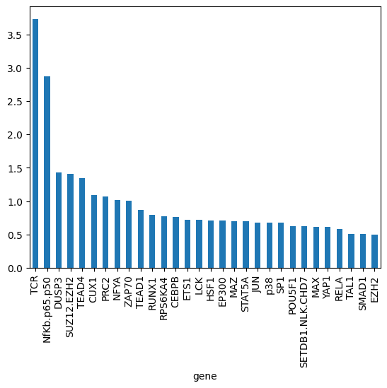
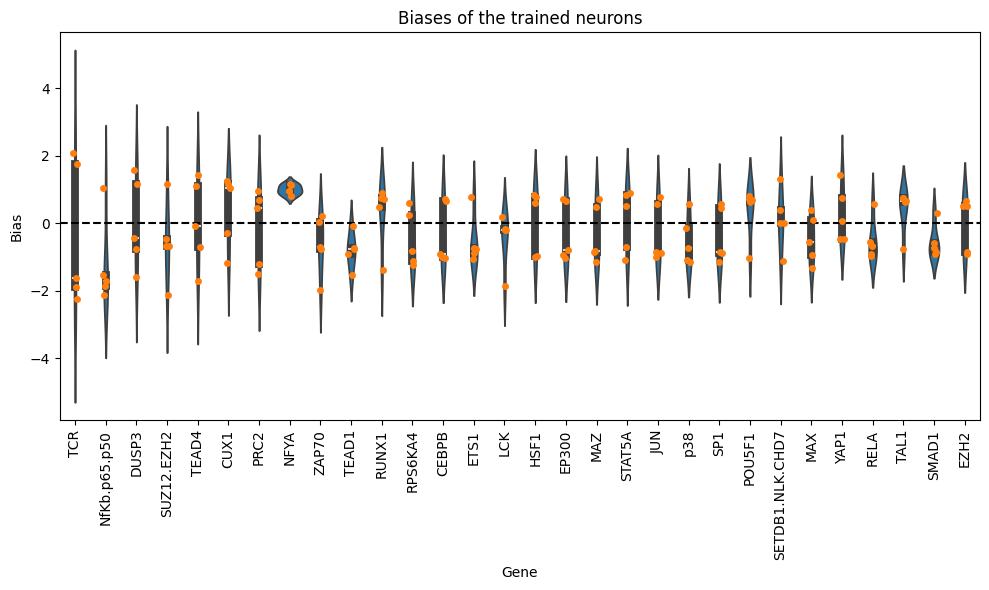
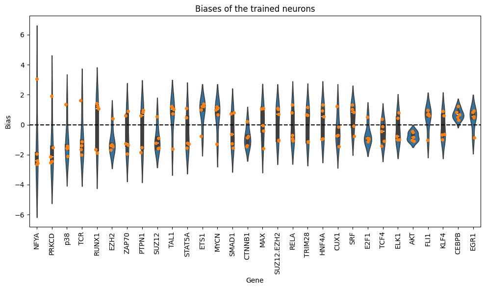
Now, we will analyze the learned biases for each of the nodes in the graph. Note that authors in the KPNN paper explain a way to extract weights for the nodes, based on the learned interactions and accounting for biases in the structure of the NN. Here we just show the learned biases of the nodes of the NN across 5 folds. Please be careful interpreting these weights.

# We collect the weights obtained in each fold


def load_biases(file="weights", folds=5):
    biases = []
    mean_inputs = []
    for i in range(5):
        model = keras.models.load_model(f"{file}_{i}.keras")
        for layer in model.layers:
            weights = layer.get_weights()
            if weights:
                biases.append((i, layer.name, weights[1][0]))
                mean_inputs.append((i, layer.name, weights[0].mean()))
    df_biases = pd.DataFrame(biases, columns=["fold", "gene", "bias"])
    df_biases["abs_bias"] = df_biases.bias.abs()
    df_biases["pow2_bias"] = df_biases.bias.pow(2)
    df_biases = df_biases.set_index(["fold", "gene"])
    return df_biases


df_biases = load_biases(file=os.path.join(temp_weights, "weights"), folds=5)
df_biases.sort_values(by="abs_bias", ascending=False).head(10)

		bias	abs_bias	pow2_bias
fold	gene
3	TCR	-2.239990	2.239990	5.017553
4	SUZ12.EZH2	-2.131501	2.131501	4.543296
2	NfKb.p65.p50	-2.116935	2.116935	4.481413
0	TCR	2.072657	2.072657	4.295907
4	ZAP70	-1.976060	1.976060	3.904812
	TCR	-1.879853	1.879853	3.533846
	LCK	-1.862840	1.862840	3.470172
	NfKb.p65.p50	-1.861053	1.861053	3.463519
1	TCR	1.772437	1.772437	3.141535
0	NfKb.p65.p50	-1.715750	1.715750	2.943798

df_biases_full = df_biases.copy().reset_index()
gene_biases_score = df_biases_full.groupby("gene")["pow2_bias"].mean().sort_values(ascending=False)
gene_biases_score

gene
TCR             3.731767
NfKb.p65.p50    2.869271
DUSP3           1.426607
SUZ12.EZH2      1.408031
TEAD4           1.342012
                  ...   
RBBP5           0.000911
CBX3            0.000815
REST            0.000393
SRY             0.000071
GATA3           0.000004
Name: pow2_bias, Length: 308, dtype: float32

gene_biases_score.head(30).plot.bar()

<Axes: xlabel='gene'>

import matplotlib.pyplot as plt
import pandas as pd
import seaborn as sns

# Get the top genes sorted by mean bias
top_genes = gene_biases_score.head(30).index

# Filter the DataFrame to include only rows with these top genes
filtered_df = df_biases_full[df_biases_full["gene"].isin(top_genes)]

plt.figure(figsize=(10, 6))
sns.violinplot(data=filtered_df, x="gene", y="bias", order=top_genes, dodge=True)
sns.stripplot(data=filtered_df, x="gene", y="bias", order=top_genes, dodge=True)
plt.xticks(rotation=90)
plt.title("Biases of the trained neurons")
plt.xlabel("Gene")
plt.ylabel("Bias")
plt.axhline(0, linestyle="--", color="k")
plt.tight_layout()

Use CORNETO for NN pruning

Now we will show how CORNETO can be used to extract a smaller, yet complete DAG from the original PKN provided by the authors. We will add input edges to each input node and an output edge through TCR to indicate which nodes are the inputs and which one the output. We will use then Acyclic Flow to find the smallest DAG comprising these nodes

G_dag = G.copy()
new_edges = []
for g in input_nn:
    new_edges.append(G_dag.add_edge((), g))
new_edges.append(G_dag.add_edge("TCR", ()))
print(G_dag.shape)

# Find small DAG. We use Acyclic Flow to find over the space of DAGs
P = cn.opt.AcyclicFlow(G_dag)
# We enforce that the input genes and the output gene are part of the solution
P += P.expr.with_flow[new_edges] == 1
# Minimize the number of active edges
P.add_objectives(sum(P.expr.with_flow), weights=1)
P.solve(solver="HIGHS", verbosity=1, max_seconds=300);

(12767, 38388)
===============================================================================
                                     CVXPY                                     
                                     v1.7.5                                    
===============================================================================
-------------------------------------------------------------------------------
                                  Compilation                                  
-------------------------------------------------------------------------------
-------------------------------------------------------------------------------
                                Numerical solver                               
-------------------------------------------------------------------------------
Running HiGHS 1.13.0 (git hash: 1bce6d5): Copyright (c) 2026 under MIT licence terms
MIP has 332945 rows; 127931 cols; 628290 nonzeros; 76776 integer variables (76776 binary)
Coefficient ranges:
  Matrix  [1e-04, 1e+04]
  Cost    [1e+00, 1e+00]
  Bound   [1e+00, 1e+00]
  RHS     [1e+00, 1e+04]
Presolving model
62024 rows, 50344 cols, 163279 nonzeros  0s
41001 rows, 42167 cols, 129201 nonzeros  0s
39345 rows, 38161 cols, 131128 nonzeros  0s
Presolve reductions: rows 39345(-293600); columns 38161(-89770); nonzeros 131128(-497162) 
Objective function is integral with scale 1

Solving MIP model with:
   39345 rows
   38161 cols (18824 binary, 0 integer, 0 implied int., 19337 continuous, 0 domain fixed)
   131128 nonzeros

Src: B => Branching; C => Central rounding; F => Feasibility pump; H => Heuristic;
     I => Shifting; J => Feasibility jump; L => Sub-MIP; P => Empty MIP; R => Randomized rounding;
     S => Solve LP; T => Evaluate node; U => Unbounded; X => User solution; Y => HiGHS solution;
     Z => ZI Round; l => Trivial lower; p => Trivial point; u => Trivial upper; z => Trivial zero

        Nodes      |    B&B Tree     |            Objective Bounds              |  Dynamic Constraints |       Work      
Src  Proc. InQueue |  Leaves   Expl. | BestBound       BestSol              Gap |   Cuts   InLp Confl. | LpIters     Time

         0       0         0   0.00%   19712           inf                  inf        0      0      0         0     0.9s
         0       0         0   0.00%   19712           inf                  inf        0      0      2     16183     1.8s
 L       0       0         0   0.00%   24925.269981    25090              0.66%     7107   5683     52     37108    15.7s

0.2% inactive integer columns, restarting
Model after restart has 39266 rows, 38118 cols (18787 bin., 0 int., 1 impl., 19330 cont., 0 dom.fix.), and 130936 nonzeros

         0       0         0   0.00%   24925.269981    25090              0.66%     5526      0      0     89730    16.1s
         0       0         0   0.00%   24925.269986    25090              0.66%     5526   5430      6    161347    31.1s

Symmetry detection completed in 6.0s
Found 2479 generator(s) and 1 full orbitope(s) acting on 2 columns
        18       0         1   0.00%   24927.270705    25090              0.65%     7860   5601     81    241495    62.4s
       112     109         2   0.00%   24999.05974     25090              0.36%     7895   5601    144    259108    74.4s
       132     108         3   0.00%   24999.05974     25090              0.36%     8073   5691    150    308729   101.8s
 T     132     103         3   0.00%   24999.05974     25078              0.31%     8087   5691    187    308729   111.2s
 T     221     182         4   0.00%   25002.04224     25075              0.29%     8278   5476    210    331347   120.2s
       346     260         6   0.00%   25004.03809     25075              0.28%     8309   5487    218    377035   137.6s
       487     415        10   0.01%   25008.0326      25075              0.27%     8389   5500    245    384729   144.7s
 L     487     293        10   0.01%   25008.0326      25067              0.24%     8424   5513    245    384785   156.8s
       499     293        11   0.01%   25008.0326      25067              0.24%     8424   5513    246    435699   163.8s
       589     387        12   0.01%   25008.03426     25067              0.24%     8483   5530    262    465438   180.1s
       632     428        12   0.01%   25008.03426     25067              0.24%     8522   5463    269    491798   196.4s
       679     473        12   0.01%   25008.03426     25067              0.24%     8569   5478    274    524273   209.9s
       717     509        12   0.01%   25008.03426     25067              0.24%     8631   5490    284    554553   222.8s
       734     508        13   0.01%   25008.03426     25067              0.24%     8748   5496    286    612051   241.5s
       825     607        14   0.01%   25008.03426     25067              0.24%     8941   5485    305    644906   257.8s

        Nodes      |    B&B Tree     |            Objective Bounds              |  Dynamic Constraints |       Work      
Src  Proc. InQueue |  Leaves   Expl. | BestBound       BestSol              Gap |   Cuts   InLp Confl. | LpIters     Time

       871     651        14   0.01%   25008.03426     25067              0.24%     9095   5498    312    649869   262.9s
       914     691        14   0.01%   25008.03426     25067              0.24%     9160   5511    316    673435   274.9s
       951     725        14   0.01%   25011.03409     25067              0.22%     9357   5524    321    690262   283.2s
      1032     800        14   0.01%   25017.03253     25067              0.20%     9294   5491    332    701864   290.0s
      1140     900        14   0.01%   25024.0294      25067              0.17%     8954   5534    343    709309   295.3s
      1182     899        34   0.01%   25038.00958     25067              0.12%     8191   5514    372    718650   300.5s
      1182     899        34   0.01%   25038.00958     25067              0.12%     8191   5514    372    718650   300.5s

Solving report
  Status            Time limit reached
  Primal bound      25067
  Dual bound        25039
  Gap               0.112% (tolerance: 0.01%)
  P-D integral      0.974082103545
  Solution status   feasible
                    25067 (objective)
                    0 (bound viol.)
                    1.31794575253e-11 (int. viol.)
                    0 (row viol.)
  Timing            300.49
  Max sub-MIP depth 7
  Nodes             1182
  Repair LPs        0
  LP iterations     718650
                    148429 (strong br.)
                    53906 (separation)
                    255356 (heuristics)
-------------------------------------------------------------------------------
                                    Summary                                    
-------------------------------------------------------------------------------

G_subdag = G_dag.edge_subgraph(P.expr.with_flow.value > 0.5)
G_dag.shape, G_subdag.shape

((12767, 38388), (12608, 25067))

rel_dag_compression = (1 - (G_subdag.num_edges / G_dag.num_edges)) * 100
print(f"KPNN edge compression (0-100%): {rel_dag_compression:.2f}%")

KPNN edge compression (0-100%): 34.70%

pruned_models, pruned_metrics = stratified_kfold(
    G_subdag,
    input_nn,
    outputs_pkn,
    file_weights=os.path.join(temp_weights, "pruned_weights"),
)

print("Validation metrics:")
for k, v in pruned_metrics.items():
    print(f" - {k}: {np.mean(v):.3f}")

Building DAG NN model with CORNETO using Keras with JAX...
 > N. inputs: 12459
 > N. outputs: 1
 > N. parameters: 12756
Compiling...
Fitting...
Weights saved to /var/folders/b4/gwkwsdb93sv11rtztqbm3l040000gn/T/tmpsvm30spu/pruned_weights_0.keras
 1/11 ━━━━━━━━━━━━━━━━━━━━ 5s 510ms/step
10/11 ━━━━━━━━━━━━━━━━━━━━ 0s 9ms/step
11/11 ━━━━━━━━━━━━━━━━━━━━ 0s 51ms/step
11/11 ━━━━━━━━━━━━━━━━━━━━ 1s 51ms/step
 > Fold 0 validation ROC-AUC=0.986
Building DAG NN model with CORNETO using Keras with JAX...
 > N. inputs: 12459
 > N. outputs: 1
 > N. parameters: 12756
Compiling...
Fitting...
Weights saved to /var/folders/b4/gwkwsdb93sv11rtztqbm3l040000gn/T/tmpsvm30spu/pruned_weights_1.keras
 1/11 ━━━━━━━━━━━━━━━━━━━━ 5s 530ms/step
10/11 ━━━━━━━━━━━━━━━━━━━━ 0s 9ms/step
11/11 ━━━━━━━━━━━━━━━━━━━━ 0s 54ms/step
11/11 ━━━━━━━━━━━━━━━━━━━━ 1s 54ms/step
 > Fold 1 validation ROC-AUC=0.977
Building DAG NN model with CORNETO using Keras with JAX...
 > N. inputs: 12459
 > N. outputs: 1
 > N. parameters: 12756
Compiling...
Fitting...
Weights saved to /var/folders/b4/gwkwsdb93sv11rtztqbm3l040000gn/T/tmpsvm30spu/pruned_weights_2.keras
 1/11 ━━━━━━━━━━━━━━━━━━━━ 5s 516ms/step
10/11 ━━━━━━━━━━━━━━━━━━━━ 0s 10ms/step
11/11 ━━━━━━━━━━━━━━━━━━━━ 0s 54ms/step
11/11 ━━━━━━━━━━━━━━━━━━━━ 1s 54ms/step
 > Fold 2 validation ROC-AUC=0.972
Building DAG NN model with CORNETO using Keras with JAX...
 > N. inputs: 12459
 > N. outputs: 1
 > N. parameters: 12756
Compiling...
Fitting...
Weights saved to /var/folders/b4/gwkwsdb93sv11rtztqbm3l040000gn/T/tmpsvm30spu/pruned_weights_3.keras
 1/11 ━━━━━━━━━━━━━━━━━━━━ 5s 529ms/step
10/11 ━━━━━━━━━━━━━━━━━━━━ 0s 9ms/step
11/11 ━━━━━━━━━━━━━━━━━━━━ 0s 55ms/step
11/11 ━━━━━━━━━━━━━━━━━━━━ 1s 55ms/step
 > Fold 3 validation ROC-AUC=0.993
Building DAG NN model with CORNETO using Keras with JAX...
 > N. inputs: 12459
 > N. outputs: 1
 > N. parameters: 12756
Compiling...
Fitting...
Weights saved to /var/folders/b4/gwkwsdb93sv11rtztqbm3l040000gn/T/tmpsvm30spu/pruned_weights_4.keras
 1/11 ━━━━━━━━━━━━━━━━━━━━ 4s 494ms/step
10/11 ━━━━━━━━━━━━━━━━━━━━ 0s 9ms/step
11/11 ━━━━━━━━━━━━━━━━━━━━ 0s 53ms/step
11/11 ━━━━━━━━━━━━━━━━━━━━ 1s 53ms/step
 > Fold 4 validation ROC-AUC=0.993
Validation metrics:
 - accuracy: 0.954
 - precision: 0.964
 - recall: 0.943
 - f1: 0.953
 - roc_auc: 0.984

df_biases_pruned = load_biases(file=os.path.join(temp_weights, "pruned_weights"), folds=5)
df_biases_pruned.sort_values(by="abs_bias", ascending=False).head(10)

		bias	abs_bias	pow2_bias
fold	gene
4	NFYA	3.065814	3.065814	9.399217
0	NFYA	-2.624697	2.624697	6.889035
3	NFYA	-2.572750	2.572750	6.619040
1	PRKCD	-2.546224	2.546224	6.483256
3	PRKCD	-2.433494	2.433494	5.921891
1	NFYA	-2.403039	2.403039	5.774594
0	PRKCD	-2.151819	2.151819	4.630327
	p38	-2.094165	2.094165	4.385529
4	TCR	-1.995883	1.995883	3.983549
2	NFYA	-1.943627	1.943627	3.777687

df_biases_prunedr = df_biases_pruned.copy().reset_index()
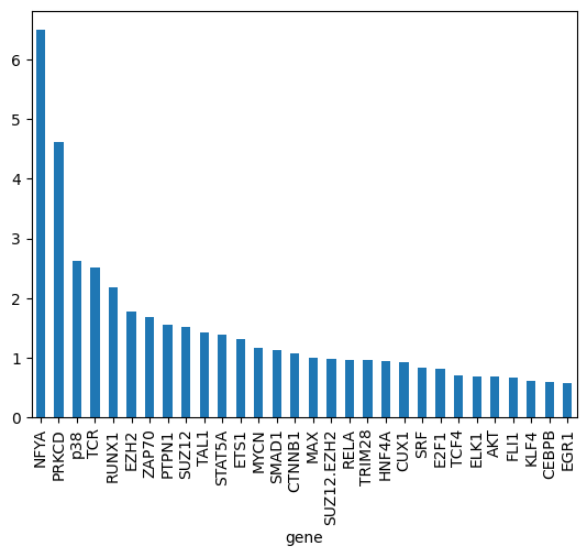
gene_biases_score = df_biases_prunedr.groupby("gene")["pow2_bias"].mean().sort_values(ascending=False)
gene_biases_score

gene
NFYA                  6.491914e+00
PRKCD                 4.609087e+00
p38                   2.618869e+00
TCR                   2.506049e+00
RUNX1                 2.171145e+00
                          ...     
ATF2                  5.205700e-03
MLL.SET.subcomplex    4.449616e-03
ZNF217                2.427842e-03
ASH2L                 1.096316e-04
GATA3                 1.853837e-07
Name: pow2_bias, Length: 149, dtype: float32

gene_biases_score.head(30).plot.bar()

<Axes: xlabel='gene'>

# Get the top genes sorted by mean bias
top_genes = gene_biases_score.head(30).index

# Filter the DataFrame to include only rows with these top genes
filtered_df = df_biases_prunedr[df_biases_prunedr["gene"].isin(top_genes)]

plt.figure(figsize=(10, 6))
sns.violinplot(data=filtered_df, x="gene", y="bias", order=top_genes, dodge=True)
sns.stripplot(data=filtered_df, x="gene", y="bias", order=top_genes, dodge=True)
plt.xticks(rotation=90)
plt.title("Biases of the trained neurons")
plt.xlabel("Gene")
plt.ylabel("Bias")
plt.axhline(0, linestyle="--", color="k")
plt.tight_layout()

param_compression = (1 - (pruned_models[0].count_params() / models[0].count_params())) * 100
print(f"Parameter compression: {param_compression:.2f}%")

Parameter compression: 51.38%

perf_degradation = (
    (np.mean(metrics["roc_auc"]) - np.mean(pruned_metrics["roc_auc"])) / np.mean(metrics["roc_auc"])
) * 100
print(
    f"Degradation in ROC-AUC after compression (positive = decrease in performance, negative = increase in performance): {perf_degradation:.2f}%"
)

Degradation in ROC-AUC after compression (positive = decrease in performance, negative = increase in performance): 0.44%