Plotting#
This guide shows how to visualize CORNETO graphs, from basic plotting to configurable styling.
It covers:
plotting a graph directly
styling edges and vertices from numeric values
using presets for common workflows
customizing themes
exporting and interoperability (DOT, pydot, NetworkX)
browser-side rendering for notebook environments
import corneto as cn
from corneto.graph import Graph

cn.info()

|
|
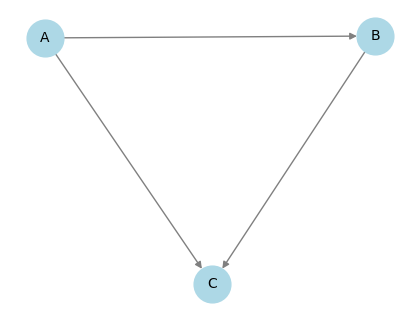
1. Basic graph visualization#
Create a graph and visualize it directly.
G = Graph(name="toy")
G.add_edge("A", "B")
G.add_edge("B", "C")
G.add_edge("A", "C")

G.plot()

2. Visual encoding from values#
Map signs and magnitudes to colors and line widths. This is useful for inspecting activities, scores, or inferred edge effects.
G.plot_values(
    edge_values=[-1, 2, 0],
    vertex_values=[1, -1, 0],
)
'digraph {\n node [fixedsize="true"];\n "A" [shape="circle", color="firebrick4", penwidth="2"];\n "B" [shape="circle", color="dodgerblue4", penwidth="2"];\n "B" [shape="circle", color="dodgerblue4", penwidth="2"];\n "C" [shape="circle"];\n "A" [shape="circle", color="firebrick4", penwidth="2"];\n "C" [shape="circle"];\n "A" -> "B" [arrowhead="normal", penwidth="5", color="dodgerblue4"];\n "B" -> "C" [arrowhead="normal", penwidth="5", color="firebrick4"];\n "A" -> "C" [arrowhead="normal", penwidth="0.25", color="black"];\n}'
You can also focus on a subset of edges.
G.plot_values(edge_values=[-1, 2, 0], edge_indexes=[0, 1])
'digraph {\n node [fixedsize="true"];\n "A" [shape="circle"];\n "B" [shape="circle"];\n "B" [shape="circle"];\n "C" [shape="circle"];\n "A" -> "B" [arrowhead="normal", penwidth="5", color="dodgerblue4"];\n "B" -> "C" [arrowhead="normal", penwidth="5", color="firebrick4"];\n}'
3. Presets for common workflows#
Presets provide sensible styling defaults with minimal code.
G.plot(
    preset="default",
    data={
        "edge_values": [-1.5, 2.0, 0.1],
        "vertex_values": [1.0, -0.5, 0.0],
    },
)

Metabolic flux visualization#
For metabolic models, metabolism rescales flux values and highlights sign and magnitude.
G_flux = Graph(name="flux-demo")
G_flux.add_edge("Glucose", "Pyruvate")
G_flux.add_edge("Pyruvate", "Lactate")
G_flux.add_edge("Pyruvate", "Acetyl-CoA")

G_flux.plot(
    preset="metabolism",
    data={
        "edge_values": [20.0, -0.2, 3.0],
        "scale": "log",
        "clip_quantil": 0.05,
    },
)

Method-aware presets and role styling#
Some presets can apply role-aware node styling when role metadata is available (for example from feature_data).
This keeps the plotting API generic while allowing method-specific defaults.
As one concrete case, preset="signaling" uses defaults such as:
input(e.g. receptors): triangleoutput(e.g. TFs): diamondinternal nodes: circle
You can still override styles explicitly via role_styles or custom_vertex_attr.
# Example: signaling preset with role metadata + custom solution variable names
G_sig = Graph(name="signaling-demo")
G_sig.add_edge("TGFBR1", "AKT1")
G_sig.add_edge("AKT1", "STAT3")

D_sig = cn.Data.from_cdict(
    {
        "sample1": {
            "TGFBR1": {"mapping": "vertex", "role": "input", "value": 1.0},
            "STAT3": {"mapping": "vertex", "role": "output", "value": -1.0},
        }
    }
)

G_sig.plot(
    preset="signaling",
    feature_data=D_sig,
    solution={"v": [1.0, 0.0, -1.0], "e": [1.0, -1.0]},
    solution_map={"vertex": "v", "edge": "e"},
)

4. Theme customization#
Override theme values to adapt colors and widths to your preferred visual style.
G.plot(
    processor="sign_magnitude",
    theme={
        "positive_color": "darkgreen",
        "negative_color": "darkorange",
        "zero_color": "gray40",
        "min_edge_width": 0.5,
        "max_edge_width": 6.0,
    },
    data={"edge_values": [-1.5, 2.0, 0.0]},
)

5. Export and interoperability#
Export DOT text or backend objects for integration with other tools.
dot_source = G.to_dot()
print(type(dot_source), dot_source.splitlines()[0])

G_pydot = G.to_dot(backend="pydot")
print(type(G_pydot))

G_graphviz = G.to_graphviz()
print(type(G_graphviz))
<class 'str'> digraph {
<class 'pydot.core.Dot'>
<class 'graphviz.graphs.Digraph'>
from IPython.display import SVG, display

display(SVG(G_pydot.create_svg()))

import matplotlib.pyplot as plt
import networkx as nx
from networkx.drawing.nx_pydot import from_pydot, graphviz_layout

G_nx = from_pydot(G.to_dot(backend="pydot"))
pos = graphviz_layout(G_nx, prog="neato")

plt.figure(figsize=(4, 3))
nx.draw(
    G_nx,
    pos,
    with_labels=True,
    arrows=True,
    node_color="lightblue",
    edge_color="gray",
    node_size=700,
    font_size=10,
)
plt.show()
6. Browser/WASM rendering#
Use renderer="wasm" in browser-based notebook environments
(e.g. marimo or Pyodide) where local Graphviz dot may be unavailable.
G.plot(renderer="wasm")
7. Custom processors#
A processor is a callable:
processor(graph, data, theme) -> (edge_attrs, vertex_attrs).
Use a custom processor when styling needs to follow domain-specific rules.
def highlight_path_processor(graph, data, theme):
    path_edges = set(data.get("path_edges", []))
    edge_attrs = {}
    for i in range(graph.num_edges):
        if i in path_edges:
            edge_attrs[i] = {"color": "purple", "penwidth": "5"}
        else:
            edge_attrs[i] = {
                "color": theme.get("zero_color", "black"),
                "penwidth": "1",
            }
    return edge_attrs, {}


G.plot(
    processor=highlight_path_processor,
    theme={"zero_color": "lightgray"},
    data={"path_edges": [0, 1]},
)
