Multi-sample CARNIVAL#
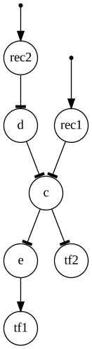
Multi-sample CARNIVAL uses CarnivalFlow to infer signaling networks for several samples or conditions together. Each sample has its own receptor inputs, TF measurements, and inferred signaling states, all on the same prior knowledge network. Inputs and measurements can differ between samples.
The joint fit balances agreement with each sample’s TF measurements against the size of the combined network. With lambda_reg > 0, an edge selected in several samples is penalized only once, encouraging the solutions to share edges. Increasing lambda_reg favors a smaller combined network, potentially at the cost of fitting the measurements. Shared edges do not require identical signaling states in every sample.
Below, we fit two conditions jointly, inspect their solutions, and compare them with independent fits. The final section applies the same approach to a single condition by treating each receptor as a separate sample with the same TF measurements.
import numpy as np
import pandas as pd

import corneto as cn

cn.info()

|
|
Toy example#
from corneto.graph import Graph

# A toy PKN signalling network
G = Graph.from_tuples(
    [
        ("rec1", 1, "a"),
        ("rec1", -1, "b"),
        ("rec1", 1, "f"),
        ("rec1", -1, "c"),
        ("rec2", 1, "b"),
        ("rec2", 1, "tf2"),
        ("b", 1, "g"),
        ("g", -1, "d"),
        ("rec2", -1, "d"),
        ("a", 1, "c"),
        ("a", -1, "d"),
        ("c", 1, "d"),
        ("c", -1, "e"),
        ("c", 1, "tf3"),
        ("e", 1, "a"),
        ("d", -1, "c"),
        ("e", 1, "tf1"),
        ("a", -1, "tf1"),
        ("d", 1, "tf2"),
        ("c", -1, "tf2"),
        ("tf1", 1, "tf2"),
        ("tf1", -1, "rec2"),
        ("tf2", 1, "rec1"),
        ("tf1", 1, "f"),
    ]
)
G.plot()

from corneto.methods.carnival import CarnivalFlow

samples = {
    "c1": {
        "rec2": {"value": 1, "mapping": "vertex", "role": "input"},
        "tf1": {"value": -2, "mapping": "vertex", "role": "output"},
        "tf2": {"value": 1, "mapping": "vertex", "role": "output"},
    },
    "c2": {
        "rec1": {"value": 1, "mapping": "vertex", "role": "input"},
        "rec2": {"value": -1, "mapping": "vertex", "role": "input"},
        "tf1": {"value": 1, "mapping": "vertex", "role": "output"},
        "tf2": {"value": -1, "mapping": "vertex", "role": "output"},
        "tf3": {"value": 3, "mapping": "vertex", "role": "output"},
    },
}

data = cn.Data.from_cdict(samples)
data
Data(n_samples=2, n_feats=[3 5])
Solving the conditions jointly#
c = CarnivalFlow(lambda_reg=1e-3)
P = c.build(G, data)

# Solve the problem using the HIGHs solver included in Scipy
P.solve(verbosity=0, solver="scipy");
Unreachable vertices for sample: 1
Unreachable vertices for sample: 0
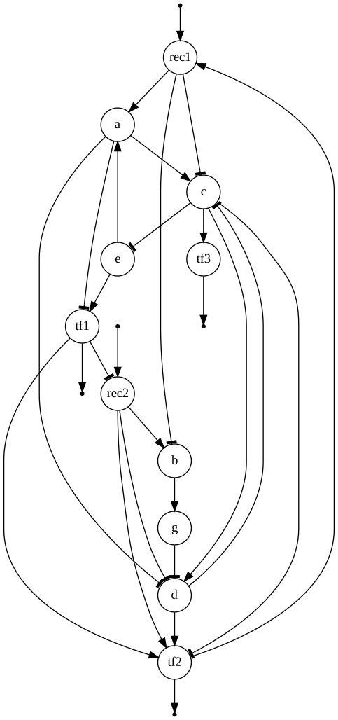
# The preprocessed G graph (flow graph)
c.processed_graph.plot()
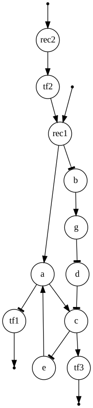
# Show the sub-graph where the signal propagates for all samples (union graph)
c.processed_graph.edge_subgraph(np.flatnonzero(P.expr.flow.value)).plot()
# Extract the values from the problem
pd.DataFrame(
    P.expr.edge_value.value,
    index=c.processed_graph.E,
    columns=["condition_1", "condition_2"],
).astype(int)
| condition_1 | condition_2 | ||
|---|---|---|---|
| (rec1) | (a) | 1 | 1 |
| (b) | 0 | 0 | |
| (c) | 0 | 0 | |
| (rec2) | (b) | 0 | 0 |
| (tf2) | 1 | -1 | |
| (b) | (g) | 0 | 0 |
| (g) | (d) | 0 | 0 |
| (rec2) | (d) | 0 | 0 |
| (a) | (c) | 0 | 1 |
| (d) | 0 | 0 | |
| (c) | (d) | 0 | 0 |
| (e) | 0 | 0 | |
| (tf3) | 0 | 1 | |
| (e) | (a) | 0 | 0 |
| (d) | (c) | 0 | 0 |
| (e) | (tf1) | 0 | 0 |
| (a) | (tf1) | -1 | 0 |
| (d) | (tf2) | 0 | 0 |
| (c) | (tf2) | 0 | 0 |
| (tf1) | (tf2) | 0 | 0 |
| (rec2) | 0 | 0 | |
| (tf2) | (rec1) | 1 | 0 |
| (tf3) | () | 0 | 0 |
| (tf1) | () | 0 | 0 |
| (tf2) | () | 0 | 0 |
| () | (rec1) | 0 | 1 |
| (rec2) | 1 | -1 |
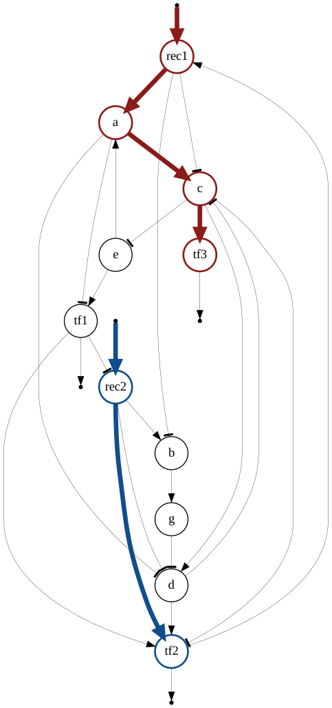
# Solution for sample 1
c.processed_graph.edge_subgraph(np.flatnonzero(P.expr.edge_has_signal.value[:, 0] > 0.5)).plot()

# Solution for sample 2
c.processed_graph.edge_subgraph(np.flatnonzero(P.expr.edge_has_signal.value[:, 1] > 0.5)).plot()

for o in P.objectives:
    print(o.value)
0.0
1.0
8.0
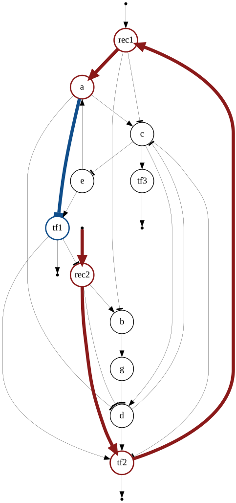
Plotting solutions on top of the PKN#
c.processed_graph.plot_values(
    vertex_values=P.expr.vertex_value.value[:, 0],
    edge_values=P.expr.edge_value.value[:, 0],
)
c.processed_graph.plot_values(
    vertex_values=P.expr.vertex_value.value[:, 1],
    edge_values=P.expr.edge_value.value[:, 1],
)
Penalizing indirect signaling rules#
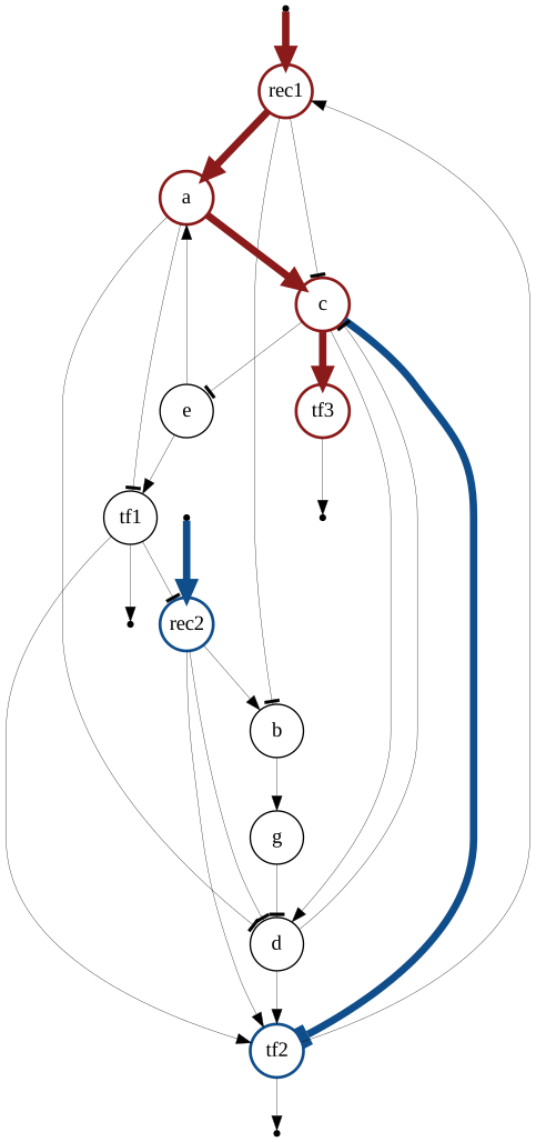
The original version of CARNIVAL treats indirect rules (A -> B, A inhibited => B inhibited, and A -| B, A inhibited => B activated) similarly that more direct rules (…). The reverse or inactive-state implications rely, in general, on additional assumptions, such as A being the sole regulator of B or the existence of efficient off-switch mechanisms, and these might be in general less reliable. To control for this, we added a tunable parameter called indirect_rule_penalty that penalizes the number of indirect rules selected in each sample
c = CarnivalFlow(lambda_reg=1e-3, indirect_rule_penalty=1)
P = c.build(G, data)
P.solve(verbosity=0, solver="scipy")

for o in P.objectives:
    print(o.name, o.value)
Unreachable vertices for sample: 1
Unreachable vertices for sample: 0
error_c1_0 0.0
penalty_indirect_rules_0 [0.]
error_c2_1 1.0
penalty_indirect_rules_1 [1.]
regularization_edge_has_signal_OR 9.0
c.processed_graph.plot_values(
    vertex_values=P.expr.vertex_value.value[:, 0],
    edge_values=P.expr.edge_value.value[:, 0],
)
c.processed_graph.plot_values(
    vertex_values=P.expr.vertex_value.value[:, 1],
    edge_values=P.expr.edge_value.value[:, 1],
)
Solving each condition independently#
To compare the joint solution with separate fits, we can run CarnivalFlow once for each condition. Each run uses only that condition’s inputs and TF measurements, so there is no shared-edge penalty linking the two solutions. The cells below solve c1 and c2 separately.
# Only c1

subset = cn.Data.from_cdict({"c1": samples["c1"]})
c = CarnivalFlow(lambda_reg=1e-3)
P = c.build(G, subset)
P.solve(verbosity=0, solver="scipy")
for o in P.objectives:
    print(o.value)

c.processed_graph.edge_subgraph(np.flatnonzero(P.expr.edge_has_signal.value)).plot()
Unreachable vertices for sample: 0
0.0
5.0
# Only c2

subset = cn.Data.from_cdict({"c2": samples["c2"]})
c = CarnivalFlow(lambda_reg=1e-3)
P = c.build(G, subset)
P.solve(verbosity=0, solver="scipy")
for o in P.objectives:
    print(o.value)

c.processed_graph.edge_subgraph(np.flatnonzero(P.expr.edge_has_signal.value)).plot()
Unreachable vertices for sample: 0
1.0
6.0
Multi-receptor integration#
A single condition can have several receptor inputs. When they are all supplied in one CARNIVAL sample, the solution may explain the TF measurements through only a subset of those receptors.
We can use the multi-sample formulation to consider each receptor separately: create one sample per receptor and give every sample the same TF measurements. These samples represent receptor-specific scenarios for the same condition, rather than separate experiments. Solving them jointly encourages a compact combined network linking the receptors to the common TF readout.
We reuse the toy network above. Both scenarios use the same measurements: tf1 and tf2 are active (+1). Only the specified receptor input changes: rec1 is active (+1) in the first scenario, and rec2 is inhibited (-1) in the second. As with the earlier joint fit, TF measurements are fitting targets, so this setup does not guarantee a path from every receptor to every TF.
shared_tf_measurements = {
    "tf1": {"value": 1, "mapping": "vertex", "role": "output"},
    "tf2": {"value": 1, "mapping": "vertex", "role": "output"},
}

receptor_scenarios = {
    "rec1_scenario": {
        "rec1": {"value": 1, "mapping": "vertex", "role": "input"},
        **shared_tf_measurements,
    },
    "rec2_scenario": {
        "rec2": {"value": -1, "mapping": "vertex", "role": "input"},
        **shared_tf_measurements,
    },
}

receptor_data = cn.Data.from_cdict(receptor_scenarios)
receptor_method = CarnivalFlow(lambda_reg=1e-3)
receptor_problem = receptor_method.build_from_data(G, receptor_data)
receptor_problem.solve(verbosity=0, solver="scipy")
Unreachable vertices for sample: 0
Unreachable vertices for sample: 0
Problem(Minimize(Expression(AFFINE, UNKNOWN, ())), [Inequality(Constant(CONSTANT, ZERO, (25,))), Inequality(Variable((25,), _flow)), Inequality(Constant(CONSTANT, ZERO, (10, 2))), Inequality(Variable((10, 2), _dag_layer)), Equality(Expression(AFFINE, UNKNOWN, (10,)), Constant(CONSTANT, ZERO, ())), Inequality(Expression(AFFINE, NONNEGATIVE, (25, 2))), Inequality(Expression(AFFINE, NONNEGATIVE, (10, 2))), Inequality(Expression(AFFINE, UNKNOWN, (21, 2))), Inequality(Expression(AFFINE, UNKNOWN, (21, 2))), Inequality(Constant(CONSTANT, NONNEGATIVE, (10, 2))), Inequality(Expression(AFFINE, NONNEGATIVE, (25, 2))), Inequality(Expression(AFFINE, NONNEGATIVE, (23, 2))), Inequality(Expression(AFFINE, NONNEGATIVE, (23, 2))), Equality(Expression(AFFINE, NONNEGATIVE, (1,)), Constant(CONSTANT, ZERO, ())), Equality(Expression(AFFINE, NONNEGATIVE, (1,)), Constant(CONSTANT, ZERO, ())), Equality(Expression(AFFINE, UNKNOWN, (1,)), Constant(CONSTANT, NONNEGATIVE, (1,))), Equality(Expression(AFFINE, NONNEGATIVE, (1,)), Constant(CONSTANT, ZERO, ())), Equality(Expression(AFFINE, NONNEGATIVE, (1,)), Constant(CONSTANT, ZERO, ())), Equality(Expression(AFFINE, UNKNOWN, (1,)), Constant(CONSTANT, NONPOSITIVE, (1,))), Inequality(Expression(AFFINE, NONNEGATIVE, (25,))), Inequality(Variable((25,), _edge_has_signal_OR, boolean=True))])
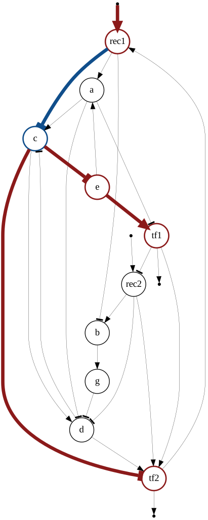
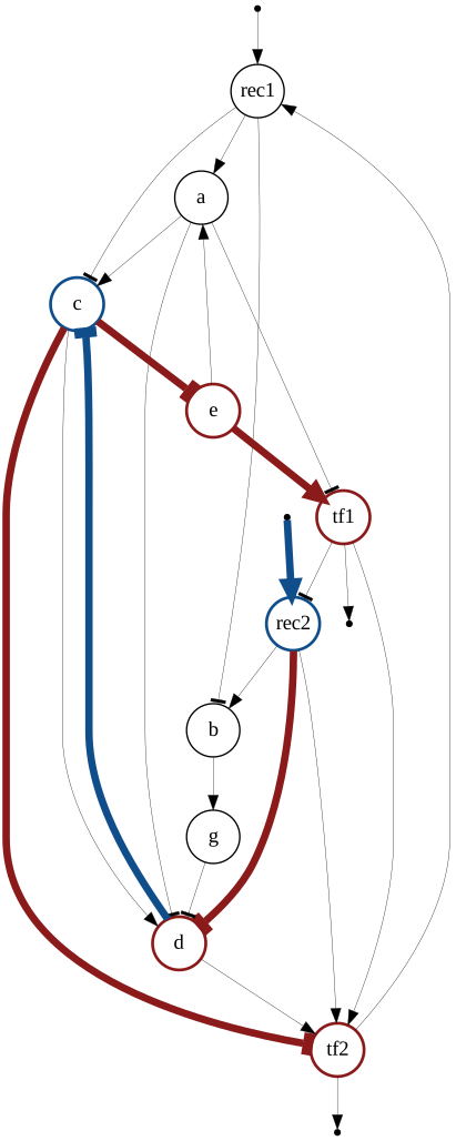
Plot each signed solution on the same network, then compare their union. The scenario columns keep the order used above: rec1_scenario first and rec2_scenario second.
from IPython.display import Markdown, display

for sample_index, sample_name in enumerate(receptor_scenarios):
    display(Markdown(f"**{sample_name.replace('_', ' ')}**"))
    display(
        receptor_method.processed_graph.plot_values(
            vertex_values=receptor_problem.expr.vertex_value.value[:, sample_index],
            edge_values=receptor_problem.expr.edge_value.value[:, sample_index],
        )
    )

selected_edges_by_sample = receptor_problem.expr.edge_has_signal.value
union_edges = np.any(selected_edges_by_sample > 0.5, axis=1)
display(Markdown("**Union of edges selected in either scenario**"))
display(receptor_method.processed_graph.edge_subgraph(np.flatnonzero(union_edges)).plot())
rec1 scenario
rec2 scenario
Union of edges selected in either scenario