Multi-condition gene expression integration#

The single-condition expression guide showed how iMAT converts expression evidence into reaction-level preferences, while the Multi-condition FBA guide explained why reaction selection should be performed jointly when shared and context-specific metabolism are the biological quantities of interest.

This guide combines those ideas without repeating their derivations. Each condition receives its own reaction scores, medium bounds, phenotype constraints, and flux vector. CORNETO then fits the condition-specific expression evidence while selecting one compact reaction union across the complete experiment.

What changes in the multi-condition formulation?#

MultiSampleIMAT.build_many accepts mappings whose first level contains condition names:

Input	Condition-specific information
`reaction_scores`	Reactions favored active (`+1`), favored inactive (`−1`), or unscored
`reaction_bounds`	Medium, perturbations, and required phenotypes
`objectives`	Optional reaction objectives

Every condition keeps a separate flux vector and a separate expression-fit objective. With lambda_reg > 0, a reaction active in one or several conditions contributes once to the union penalty. Reuse is therefore encouraged, but conflicting or condition-specific expression evidence can still select different pathways.

This is the same union-level coupling introduced in Multi-condition FBA, now applied while every condition also fits its own expression evidence. The joint model does not average expression profiles and does not force equal fluxes. Reaction-level agreement must therefore be inspected alongside the inferred network: an unmatched score can reveal tension between expression, network feasibility, phenotype constraints, and shared regularization.

from contextlib import redirect_stdout
from io import StringIO

import numpy as np
import pandas as pd
from cobra.io import load_model

from corneto.io import cobra_model_to_graph
from corneto.methods import MultiSampleIMAT

with redirect_stdout(StringIO()):
    model = load_model("textbook")

G = cobra_model_to_graph(model)
reaction_ids = list(G.get_attr_from_edges("id"))
reaction_index = {reaction_id: i for i, reaction_id in enumerate(reaction_ids)}
biomass_id = "Biomass_Ecoli_core"

Example: aerobic respiration and anaerobic fermentation#

We ask:

Which reactions form a shared expression-consistent program for growth on glucose, and which distinguish aerobic respiration from anaerobic ethanol fermentation?

The example uses two synthetic expression contexts in the E. coli core model. Both grow on glucose. Oxygen is available only in the aerobic condition, and biomass is fixed at approximately 60% of the maximum supported by each environment. The fixed phenotypes keep the independent and joint comparisons biologically equivalent.

We start from reaction scores, the advanced interface introduced at the end of the single-condition guide. In a real workflow these scores could be produced from expression measurements and GPR rules with evaluate_gpr_expression or supplied by another curated mapping procedure.

Define condition-specific reaction evidence#

The aerobic profile supports respiration and pyruvate oxidation while arguing against fermentation. The anaerobic profile supports ethanol formation while arguing against oxygen-dependent respiration and lactate production.

To make model–data disagreement visible, the synthetic anaerobic profile deliberately classifies PFL as low even though pyruvate-formate lyase provides the route from pyruvate to acetyl-CoA and formate in the selected fermentative state. This controlled conflict lets us distinguish a reaction that is fitted from one that remains active despite low-expression evidence.

condition_names = ["glucose aerobic", "glucose anaerobic"]

reaction_scores = {
    "glucose aerobic": {
        "CYTBD": 1.0,
        "NADH16": 1.0,
        "PDH": 1.0,
        "CS": 1.0,
        "ATPS4r": 1.0,
        "PFL": -1.0,
        "LDH_D": -1.0,
        "ACALD": -1.0,
        "ALCD2x": -1.0,
    },
    "glucose anaerobic": {
        "PFL": -1.0,
        "ACALD": 1.0,
        "ALCD2x": 1.0,
        "CYTBD": -1.0,
        "NADH16": -1.0,
        "PDH": -1.0,
        "LDH_D": -1.0,
    },
}

score_table = pd.DataFrame(reaction_scores).fillna(0.0)
score_table.index.name = "reaction"
score_table

	glucose aerobic	glucose anaerobic
reaction
CYTBD	1.0	-1.0
NADH16	1.0	-1.0
PDH	1.0	-1.0
CS	1.0	0.0
ATPS4r	1.0	0.0
PFL	-1.0	-1.0
LDH_D	-1.0	-1.0
ACALD	-1.0	1.0
ALCD2x	-1.0	1.0

Define the media and required phenotypes#

A negative exchange lower bound allows uptake. Biomass is fixed rather than maximized because expression agreement and shared reaction selection are the objectives of this analysis.

biomass_targets = {
    "glucose aerobic": 0.50,
    "glucose anaerobic": 0.12,
}

reaction_bounds = {
    "glucose aerobic": {
        "EX_glc__D_e": (-10.0, 1000.0),
        "EX_o2_e": (-20.0, 1000.0),
        biomass_id: (biomass_targets["glucose aerobic"], biomass_targets["glucose aerobic"]),
    },
    "glucose anaerobic": {
        "EX_glc__D_e": (-10.0, 1000.0),
        "EX_o2_e": (0.0, 1000.0),
        biomass_id: (biomass_targets["glucose anaerobic"], biomass_targets["glucose anaerobic"]),
    },
}

pd.DataFrame(
    {
        "glucose lower bound": {condition: bounds["EX_glc__D_e"][0] for condition, bounds in reaction_bounds.items()},
        "oxygen lower bound": {condition: bounds["EX_o2_e"][0] for condition, bounds in reaction_bounds.items()},
        "fixed biomass": biomass_targets,
    }
)

	glucose lower bound	oxygen lower bound	fixed biomass
glucose aerobic	-10.0	-20.0	0.50
glucose anaerobic	-10.0	0.0	0.12

Balance expression evidence across conditions#

Before coupling conditions, compare their total evidence weight. Without scaling, a condition with more scored reactions or larger score magnitudes contributes more to the joint objective. The shared sparsity penalty can then overwhelm a weakly weighted condition, especially when zero flux is feasible.

MultiSampleIMAT(scale=True) applies L1 normalization independently within each condition:

\[ \widetilde{w}_{r,c} = 100\,\frac{w_{r,c}}{\sum_j |w_{j,c}|}. \]

The signs and relative weights within a condition are preserved, while the absolute weights sum to 100. Each condition therefore has the same maximum expression-mismatch budget.

The value 100 is not mathematically special: normalizing to 1 and dividing lambda_reg by 100 would define the same trade-off. A budget of 100 usually keeps individual objective coefficients closer to order one when tens or hundreds of reactions are scored, avoiding unnecessarily tiny coefficients in the MILP.

Scaling and phenotype constraints solve different problems:

scaling balances the influence of expression evidence across conditions;
phenotype constraints prevent biologically required conditions from collapsing to a zero or otherwise trivial flux state.

Use scaling when score ranges or expression coverage differ for technical reasons. Leave scores unscaled when their absolute magnitudes are already comparable and intentionally encode confidence across conditions.

After scaling, compare the objective scales explicitly. For \(R\) model reactions, the expression-mismatch term is bounded by 100 per condition, while the union penalty is bounded by \(\lambda R\). If \(\lambda R\) approaches 100, sparsity can compete with an entire condition’s evidence budget. Collapse can occur earlier because an all-zero condition mismatches only its positive evidence; low-expression evidence already favors zero flux.

Objective scaling does not correct loose big-M constraints. iMAT activity indicators depend on reaction flux bounds, so finite, biologically meaningful bounds are also important for MILP numerical stability and performance.

eps = 1e-3
lambda_reg = 0.01
activity_tolerance = eps * (1 - eps)

score_weight_comparison = pd.DataFrame(
    {
        "unscaled absolute score sum": score_table.abs().sum(),
        "absolute score sum with scale=True": 100.0,
    }
)
score_weight_comparison

	unscaled absolute score sum	absolute score sum with scale=True
glucose aerobic	9.0	100.0
glucose anaerobic	7.0	100.0

pd.Series(
    {
        "expression-mismatch budget per condition": 100.0,
        "regularization cost per union reaction": lambda_reg,
        "maximum union penalty in this model": lambda_reg * len(reaction_ids),
    },
    name="objective scale",
)

expression-mismatch budget per condition    100.00
regularization cost per union reaction        0.01
maximum union penalty in this model           0.95
Name: objective scale, dtype: float64

Independent iMAT as a reference#

We first solve each condition separately with the same small reaction-count penalty used below. These runs fit each expression profile independently and provide the post-hoc union against which the joint analysis will be compared.

independent_fluxes = {}

for condition in condition_names:
    problem = MultiSampleIMAT(eps=eps, lambda_reg=lambda_reg, scale=True).build(
        G,
        reaction_scores=reaction_scores[condition],
        reaction_bounds=reaction_bounds[condition],
    )
    problem.solve(solver="highs")
    independent_fluxes[condition] = np.asarray(problem.expr.flow.value)

independent_fluxes = pd.DataFrame(independent_fluxes, index=reaction_ids)
independent_activity = independent_fluxes.abs() > activity_tolerance

pd.DataFrame(
    {
        "biomass": independent_fluxes.loc[biomass_id],
        "active reactions": independent_activity.sum(),
    }
)

	biomass	active reactions
glucose aerobic	0.50	45
glucose anaerobic	0.12	45

Solve both expression contexts jointly#

The scientific inputs have the same readable structure as the independent calls. build_many creates one flux column per named condition, and lambda_reg now penalizes their reaction union.

joint_problem = MultiSampleIMAT(
    eps=eps,
    lambda_reg=lambda_reg,
    scale=True,
).build_many(
    G,
    reaction_scores=reaction_scores,
    reaction_bounds=reaction_bounds,
)
joint_problem.solve(solver="highs")

joint_fluxes = pd.DataFrame(
    np.asarray(joint_problem.expr.flow.value),
    index=reaction_ids,
    columns=condition_names,
)
joint_activity = joint_fluxes.abs() > activity_tolerance

assert joint_problem.expr.flow.value.shape == (G.num_edges, len(condition_names))

Inspect reaction-level expression agreement#

Each condition must reach its fixed biomass. A positive reaction score is fitted when the reaction is active; a negative score is fitted when it is inactive. In the original iMAT formulation, these agreements contribute to a discrete consistency score. They are better described as fits and mismatches than as continuous residuals.

fit_rows = []
fit_details = []

for condition in condition_names:
    scores = pd.Series(reaction_scores[condition])
    joint_scored_activity = joint_activity.loc[scores.index, condition]
    independent_scored_activity = independent_activity.loc[scores.index, condition]
    joint_fitted = ((scores > 0) & joint_scored_activity) | ((scores < 0) & ~joint_scored_activity)
    independent_fitted = ((scores > 0) & independent_scored_activity) | (
        (scores < 0) & ~independent_scored_activity
    )

    for reaction_id in scores.index:
        fit_details.append(
            {
                "condition": condition,
                "reaction": reaction_id,
                "reaction score": scores[reaction_id],
                "expected": "active" if scores[reaction_id] > 0 else "inactive",
                "joint flux": joint_fluxes.loc[reaction_id, condition],
                "joint state": "active" if joint_scored_activity[reaction_id] else "inactive",
                "fitted independently": bool(independent_fitted[reaction_id]),
                "fitted jointly": bool(joint_fitted[reaction_id]),
            }
        )

    fit_rows.append(
        {
            "condition": condition,
            "biomass": joint_fluxes.loc[biomass_id, condition],
            "active reactions": int(joint_activity[condition].sum()),
            "evidence fitted": f"{int(joint_fitted.sum())}/{len(scores)}",
            "not fitted": int((~joint_fitted).sum()),
        }
    )

    assert np.isclose(joint_fluxes.loc[biomass_id, condition], biomass_targets[condition])

fit_summary = pd.DataFrame(fit_rows).set_index("condition")
fit_details = pd.DataFrame(fit_details).set_index(["reaction", "condition"])
fit_summary

	biomass	active reactions	evidence fitted	not fitted
condition
glucose aerobic	0.50	45	9/9	0
glucose anaerobic	0.12	47	6/7	1

A condition-by-reaction agreement matrix is especially useful in multi-condition analyses. It separates reactions that were not scored from scored reactions that the network could or could not fit.

all_scored_reactions = score_table.index
fit_matrix = pd.DataFrame("not scored", index=all_scored_reactions, columns=condition_names)

for (reaction_id, condition), row in fit_details.iterrows():
    fit_matrix.loc[reaction_id, condition] = "fitted" if row["fitted jointly"] else "not fitted"

fit_matrix

	glucose aerobic	glucose anaerobic
reaction
CYTBD	fitted	fitted
NADH16	fitted	fitted
PDH	fitted	fitted
CS	fitted	not scored
ATPS4r	fitted	not scored
PFL	fitted	not fitted
LDH_D	fitted	fitted
ACALD	fitted	fitted
ALCD2x	fitted	fitted

The mismatch table should be examined before interpreting shared and condition-specific pathways. A reaction mismatched both independently and jointly points to expression–feasibility tension within that condition. A reaction fitted independently but mismatched only in the joint model instead points to a trade-off introduced by shared regularization.

Expression is evidence about the likelihood of reaction activity, not a measurement of activity or flux. The original iMAT paper reports a central role for post-transcriptional regulation and uses disagreements between expression and predicted activity to generate hypotheses about regulation beyond transcript abundance. Possible mechanisms include protein translation or degradation, phosphorylation and other post-translational effects, and metabolite-level control such as substrate availability and allosteric regulation. A disagreement can also arise from expression thresholds, GPR mapping, missing or incorrect model reactions, medium composition, or an imposed phenotype. iMAT alone cannot distinguish these explanations.

mismatches = fit_details[~fit_details["fitted jointly"]].copy()

assert list(mismatches.index) == [("PFL", "glucose anaerobic")]
assert not mismatches.iloc[0]["fitted independently"]
mismatches

		reaction score	expected	joint flux	joint state	fitted independently	fitted jointly
reaction	condition
PFL	glucose anaerobic	-1.0	inactive	12.736625	active	False	False

PFL is the only unmatched reaction. It is classified as low but remains active in both the independent and joint anaerobic solutions. This is not caused by cross-condition coupling: under the imposed anaerobic growth phenotype and high ethanol evidence, the selected network uses PFL to supply acetyl-CoA and formate.

In real data, this would be a hypothesis-generating result—not proof that PFL is active despite low expression, and not proof of post-translational regulation. The first checks should separate two broad possibilities:

biology not captured by transcript abundance, including enzyme abundance or modification and metabolite-level regulation;
data or model assumptions, including thresholds, GPR rules, network completeness, medium bounds, and the required phenotype.

Proteomics, enzyme-activity, metabolomics, or flux measurements are needed to discriminate among these explanations.

What did joint inference change?#

The independent solutions are compared only after both optimizations have finished. The joint solution considers reuse while selecting the flux states, producing a smaller union and a larger internally consistent shared set.

independent_union = independent_activity.any(axis=1)
independent_shared = independent_activity.all(axis=1)
joint_union = joint_activity.any(axis=1)
joint_shared = joint_activity.all(axis=1)

selection_comparison = pd.DataFrame(
    {
        "shared reactions": {
            "independent inference, compared afterward": int(independent_shared.sum()),
            "one joint inference": int(joint_shared.sum()),
        },
        "reaction union": {
            "independent inference, compared afterward": int(independent_union.sum()),
            "one joint inference": int(joint_union.sum()),
        },
    }
)

assert joint_union.sum() < independent_union.sum()
assert joint_shared.sum() > independent_shared.sum()
selection_comparison

	shared reactions	reaction union
independent inference, compared afterward	34	56
one joint inference	40	52

Shared and condition-specific metabolism#

As in Multi-condition FBA, categories are derived from the joint activity matrix. With two conditions, every reaction in the union is either shared, aerobic-specific, or anaerobic-specific.

reaction_groups = pd.Series("inactive", index=reaction_ids, name="usage group")
reaction_groups.loc[joint_shared] = "shared"
reaction_groups.loc[joint_activity["glucose aerobic"] & ~joint_activity["glucose anaerobic"]] = (
    "glucose aerobic only"
)
reaction_groups.loc[~joint_activity["glucose aerobic"] & joint_activity["glucose anaerobic"]] = (
    "glucose anaerobic only"
)

group_table = (
    reaction_groups[joint_union]
    .groupby(reaction_groups[joint_union], sort=False)
    .agg(
        reactions="size",
        reaction_ids=lambda values: ", ".join(values.index),
    )
)

assert int(group_table["reactions"].sum()) == int(joint_union.sum())
group_table

	reactions	reaction_ids
usage group
glucose anaerobic only	7	ACALD, ALCD2x, ETOHt2r, EX_etoh_e, EX_for_e, F...
shared	40	ACKr, ACONTa, ACONTb, ACt2r, ATPM, ATPS4r, Bio...
glucose aerobic only	5	CYTBD, EX_o2_e, NADH16, O2t, PDH

Biological interpretation#

Usage group	Characteristic reactions	Interpretation
Shared	`GLCpts`, `PFK`, `GAPD`, `ENO`, `PYK`, biomass	Central glucose utilization and precursor production required in both states
Glucose aerobic only	`EX_o2_e`, `O2t`, `CYTBD`, `NADH16`, `PDH`	Oxygen uptake, respiratory electron transfer, and oxidative pyruvate metabolism
Glucose anaerobic only	`PFL`, `FORti`, `EX_for_e`, `ACALD`, `ALCD2x`, `ETOHt2r`, `EX_etoh_e`	Pyruvate-formate cleavage followed by formate and ethanol secretion

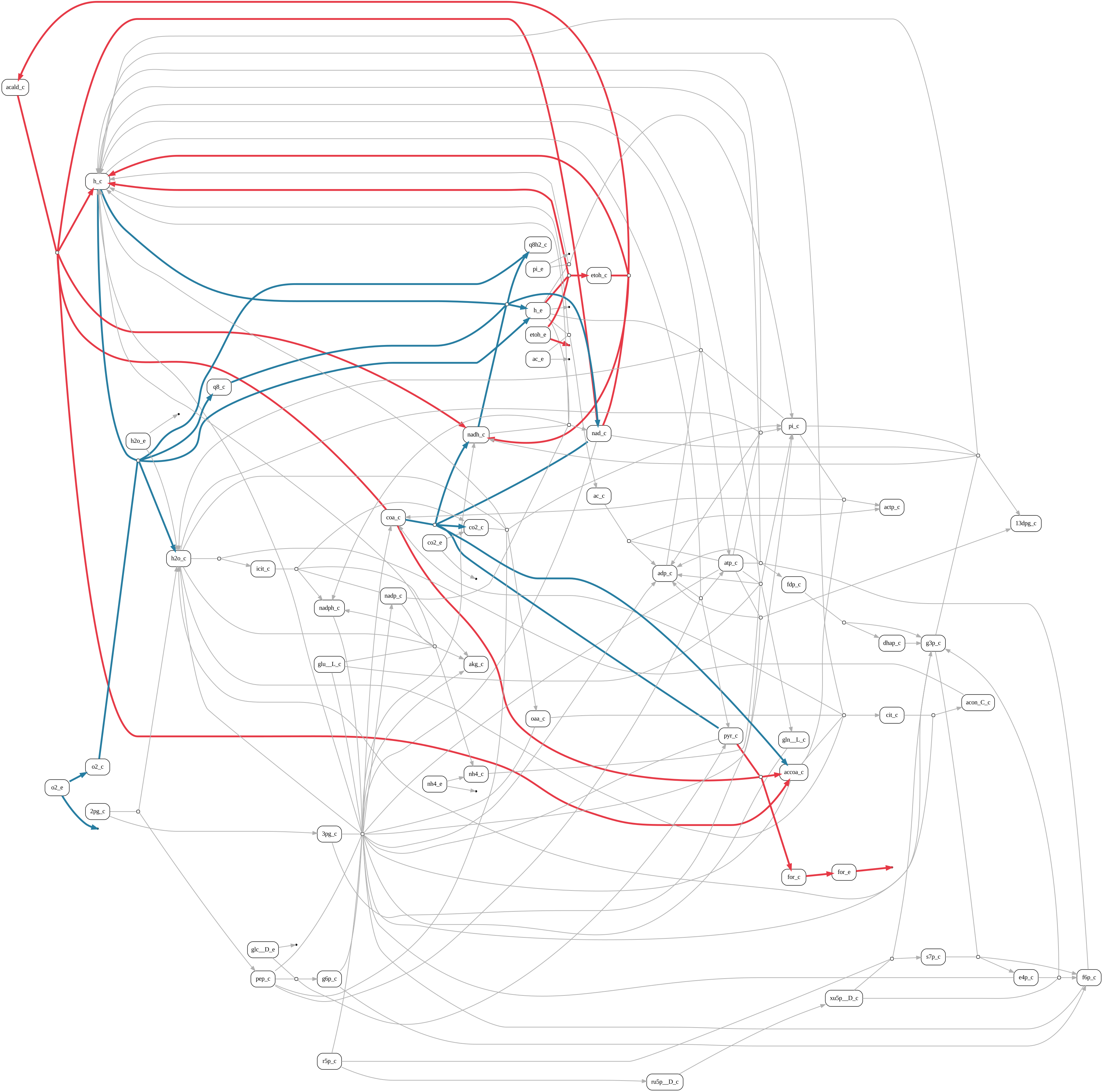
Most condition-specific reactions agree with the supplied evidence; PFL is the explicit exception identified by the mismatch analysis. The inferred sets also include the transport and exchange reactions required to complete each biological route. That is an advantage of network inference over listing high-expression reactions alone: the output is a stoichiometrically connected hypothesis that makes conflicting evidence visible.

As noted in the Multi-condition FBA guide, shared activity does not imply equal magnitude or direction. For example, ATPS4r is active in both selected states but carries flux in opposite directions in this solution.

Visualize the jointly inferred network#

The plot shows the complete joint union. Shared reactions are gray, aerobic-specific reactions are blue, and anaerobic-specific reactions are red.

Usage group	Color
Shared	Gray
Glucose aerobic only	Blue
Glucose anaerobic only	Red

group_colors = {
    "shared": "#b0b0b0",
    "glucose aerobic only": "#277da1",
    "glucose anaerobic only": "#e63946",
}

selected_reactions = np.flatnonzero(joint_union.to_numpy())
joint_network = G.edge_subgraph(selected_reactions)
edge_style = {}

for displayed_index, original_index in enumerate(selected_reactions):
    reaction_id = reaction_ids[original_index]
    group = reaction_groups[reaction_id]
    edge_style[displayed_index] = {
        "color": group_colors[group],
        "penwidth": "1.5" if group == "shared" else "4",
    }

joint_network.plot(
    graph_attr={"rankdir": "LR"},
    node_attr={
        "fixedsize": "false",
        "shape": "box",
        "style": "rounded",
        "margin": "0.05,0.03",
    },
    custom_edge_attr=edge_style,
)

../../_images/329d62a87e66c90462ef6cc0453d8eeeb05b1b1b48b93fb4ef8bab8cae4ab4e3.svg

Interpretation and limitations#

By fitting the conditions together, we can compare them against the same metabolic solution. The model reuses reactions when it can, but still keeps the respiratory pathway in the aerobic condition and fermentation in the anaerobic condition. This is different from averaging the expression profiles or comparing networks inferred in separate runs.

The fit table is an important part of the biological interpretation. It shows where the expression data support the selected network and where the model cannot satisfy both the expression evidence and the metabolic constraints. Comparing the independent and joint fits also reveals whether a mismatch was already present in one condition or appeared when the conditions were analyzed together.

Keep in mind that RNA abundance does not directly measure enzyme activity or flux. Protein abundance, post-translational regulation, and metabolite-level control can all separate expression from metabolic activity. A mismatch is therefore something to investigate, not evidence for a particular regulatory mechanism.

In practice, it is worth checking different expression thresholds and comparing the joint result with the independently inferred networks. Shared reactions may still carry different fluxes—or even operate in opposite directions—and alternative solutions may exist. The choice of lambda_reg also matters: larger values favor more reaction reuse, but can eventually outweigh weaker expression evidence.

The synthetic profiles isolate the multi-condition formulation. For a workflow using measured expression data, continue with the context-specific metabolic omics tutorial.